Machine Learning as a Coordination Layer for AI Infrastructure
Helicyn's full technical report: the coordination framework, simulator methodology, seven scheduling policies across six scenarios, results, figures, and discussion. All findings are simulated, research/prototype, and assumption-bound.
1. Abstract
The next constraint on artificial intelligence may not be model capability but the coordination of the physical infrastructure needed to power, cool, and operate large-scale computation. As cloud computing, AI training, and large-scale inference grow more common, data centers are no longer passive back-end facilities. They are becoming active nodes in a wider infrastructure system, shaped continuously by workload demand, GPU availability, thermal headroom, electricity prices, carbon intensity, cooling capacity, and regional grid conditions. In the United States alone, data center electricity use reached 176 TWh in 2023 and is projected to rise to 325–580 TWh by 2028, driven partly by the rapid deployment of GPU-accelerated AI servers and partly by uncertainty about future operating practices (Shehabi et al., 2024). Existing research shows that machine learning can improve individual parts of this system: neural networks can model cooling performance from operational sensor data, learning-based resource managers can forecast demand and guide provisioning, and reinforcement-learning-style controllers can improve sequential decisions under changing workload and thermal conditions (Gao, n.d.; Ilager & Buyya, 2021; Ilager & Buyya, 2024). The central limitation is that these methods usually act as isolated optimization tools rather than connected layers of a single coordinated system. Workload forecasting, scheduling, consolidation, power management, thermal-aware placement, cooling control, and liquid cooling are not separate problems in practice; they are coupled, interdependent decisions within one operational hierarchy. This paper argues that energy efficiency, thermal stability, and resource utilization are emergent properties of coordinating workloads, regions, facilities, and local control systems together. Machine learning in this field should therefore be understood not only as an optimization method, but as a coordination layer for increasingly interconnected AI infrastructure. To support this argument, the paper proposes a four-stage hierarchical framework: detection, coordination, optimization, and verification. Within this framework, operators remain in control while machine-learning systems first assess constraints, then recommend actions, coordinate across layers, and finally verify outcomes. To test the argument concretely, the paper pairs this framework with a reproducible, simulator-based evaluation that runs seven scheduling policies across six operating scenarios and five random seeds, using public workload, grid, carbon, and weather data. The results are deliberately modest and specific. No single policy dominates every objective. Consolidation produces the largest efficiency gains, cutting facility energy, carbon, and cost by roughly 8% by reclaiming idle server capacity, while an integrated multi-objective policy does not reduce energy outright but shifts the operating point toward lower carbon and thermal risk at the cost of higher energy and more deadline misses. Read together, these findings support the coordination framing precisely because they expose tradeoffs that isolated optimization hides. The paper makes four contributions: a hierarchical framework that reframes machine learning for AI infrastructure as coordination rather than isolated optimization, a structured synthesis of technical mechanisms across the stack, a reproducible methodology for evaluating cross-layer policies on public data, and comparative evidence that coordination manages tradeoffs rather than eliminating them. The evaluated integrated policy is a fixed-weight heuristic controller inside an ML-ready architecture, not a production-proven autonomous system.
2. Introduction
2.1 Problem Context
Data centers are quickly becoming the physical foundation of modern digital life. Search engines, cloud storage, video streaming, enterprise software, mobile applications, and now large-scale artificial intelligence all depend on facilities that run continuously. What was once treated as background technical infrastructure has moved into the spotlight, because the growth of AI workloads has raised demand for servers, accelerators, networking, cooling, power delivery, and grid capacity, turning data centers into a strategic energy and coordination concern. Barroso et al. (2019) describe this shift through the idea of a warehouse-scale computer: the data center should not be seen as a collection of machines, but as one enormous computer whose hardware, software, networking, power systems, and cooling systems operate together.
This systems-level view matters more as AI reshapes the structure of data center demand. Traditional cloud workloads already required large-scale infrastructure, but AI training and inference raise both the density and the variability of computation. GPU-accelerated servers draw large amounts of power and generate even larger amounts of concentrated heat, which demands tighter coordination between workload placement, networking, thermal limits, and cooling capacity. The 2024 Lawrence Berkeley National Laboratory report finds that U.S. data centers consumed 176 TWh of electricity in 2023, or 4.4% of total U.S. electricity consumption, after a period in which efficiency gains had kept growth relatively flat (Shehabi et al., 2024). The same report projects that U.S. data center electricity use could reach 325–580 TWh by 2028, or 6.7%–12.0% of total U.S. consumption, depending on GPU shipments, AI server utilization, operational practices, and cooling efficiency (Shehabi et al., 2024).
The problem, then, is not simply that data centers use a large amount of electricity or that cooling systems are inefficient. The deeper challenge is that AI infrastructure is becoming a system of interconnected constraints. AI workloads vary in flexibility: some inference workloads are latency-sensitive and must run immediately, while training, batch processing, and model evaluation can often shift across time or location. Regions differ in power prices, grid conditions, renewable availability, and carbon intensity. Facilities differ in available capacity, thermal headroom, cooling efficiency, hardware mix, and operational risk. Cooling systems also respond on slower timescales than compute systems; a workload can be moved or rescheduled quickly, but thermal conditions, chilled-water loops, and facility-level cooling behavior change more gradually.
These layers interact. Moving a workload from one cluster to another is not only a scheduling decision. It changes GPU utilization, rack-level heat generation, local hotspot risk, facility power demand, cooling load, and possibly exposure to different electricity prices or carbon intensity. Raising a cooling setpoint may cut chiller energy, but it also reduces thermal safety margins and limits where future workloads can be placed. Consolidating workloads may improve server utilization while creating localized heat density that raises cooling demand or hardware risk. Spreading workloads may reduce hotspots but increase the number of active servers. A decision that looks efficient inside one subsystem can turn out to be inefficient across the full infrastructure stack.
Machine learning is promising here because these relationships are too complex for static rules alone. Gao (n.d.) argues that modern data centers contain many mechanical, electrical, and control systems with nonlinear relationships that resist optimization through traditional engineering formulas. His Google study showed that a neural network trained on operational data could predict power usage effectiveness with low error, demonstrating that machine learning can use existing sensor data to model data center performance and guide efficiency improvements. Ilager and Buyya (2021, 2024) extend this argument beyond cooling, framing cloud data centers as complex cyber-physical systems in which resource management spans provisioning, scheduling, workload placement, power management, cooling control, and monitoring.
But the value of machine learning is not only its ability to optimize individual systems. Its larger contribution is coordinating decisions across layers. In AI infrastructure, work is the first control surface. Before a facility adjusts cooling setpoints, shifts power states, or changes local thermal controls, the system should ask where and when the work should run at all. This reverses the usual framing. Local optimization remains necessary, but it belongs at the end of a broader hierarchy rather than at the start. Energy efficiency emerges not only from improving a cooling system, but from coordinating workload demand, regional capacity, facility constraints, and local control actions.
2.2 Research Gap
The literature offers strong evidence that machine learning can improve data center efficiency, yet most existing approaches remain fragmented. Cooling optimization, thermal-aware scheduling, resource provisioning, workload forecasting, workload consolidation, power capping, DVFS, renewable-energy scheduling, and liquid cooling tend to be studied as separate technical domains. This separation makes research easier to evaluate, but it does not match the operating reality of AI infrastructure. In practice these mechanisms are not independent solutions. They are interconnected layers of a single coordinated system.
Ilager and Buyya (2021) explicitly identify the need for integrated, energy- and thermal-aware resource management, since computing and cooling are traditionally managed separately even though they strongly affect each other. Their survey shows that optimizing one subsystem in isolation can create unintended consequences elsewhere; raising computing utilization, for instance, may improve server efficiency while producing hotspots that increase cooling energy costs. The 2024 review reaches a similar conclusion from a machine-learning perspective: data-driven resource management is necessary because cloud data centers contain complex interactions, heterogeneous workloads, nonlinear parameters, and too many possible configurations for manual tuning (Ilager & Buyya, 2024).
Current research therefore demonstrates two things at once. First, machine learning is technically useful for specific optimization tasks. Cooling has some of the strongest evidence for deployment, particularly in Google’s neural-network-based PUE modeling work (Gao, n.d.). Workload prediction, scheduling, consolidation, DVFS, power-aware control, and thermal-aware placement also show meaningful technical promise. Second, the literature remains limited because many approaches optimize within a single domain or a single facility. A model may forecast workload demand without coordinating with energy prices. A scheduler may place workloads without considering regional carbon intensity. A cooling controller may tune setpoints without knowing whether flexible work could have been shifted away from a thermally constrained facility. A power-aware system may reduce server energy without accounting for downstream cooling effects.
The missing layer is coordination. Existing work does integrate some pairs of mechanisms: DVFS with consolidation, workload placement with cooling, or workflow scheduling with renewable availability. What remains scarce is an operator-facing hierarchy that connects workload flexibility, fleet-level regional coordination, facility thermal and power constraints, local cooling and power controls, and post-action verification within one framework. Little existing work treats workloads, fleets, regions, power conditions, thermal behavior, and facility-level controls as parts of a unified hierarchical system with a verification loop. This gap matters especially for AI infrastructure because the unit of optimization is expanding. The relevant system is no longer always a single data center. Increasingly it is a fleet of AI infrastructure in which individual data centers function as nodes within a larger network of capacity, energy, and thermal constraints. Workload placement, regional balancing, facility response, and local cooling behavior have to be considered together.
This paper addresses that gap by arguing that machine learning should be understood not only as a tool for local optimization, but as a coordination layer for AI infrastructure. The aim is not to replace operators or claim fully autonomous control. In production environments operators must stay in control, because downtime, overheating, SLA violations, and unsafe control actions can be extremely expensive. The more practical near-term role for machine learning is to detect constraints, coordinate possible responses, recommend actions, and verify whether those actions achieved the intended result. In this framing, machine learning becomes an operator-facing intelligence layer rather than a black-box replacement for facility or infrastructure teams.
This shift also changes how the research problem should be evaluated. The key question is not only whether a model can reduce cooling energy, predict workload demand, or improve scheduling in isolation. The more important question is whether these capabilities can be connected into a hierarchy that produces better system-level outcomes. Energy efficiency, thermal stability, and resource utilization should not be treated as independent objectives. They are emergent properties of coordinating decisions across workload, regional, facility, and local control.
2.3 Proposed Framework
This paper proposes a hierarchical coordination framework for AI infrastructure, built on a single principle: coordinate first, optimize everywhere. Workloads sit at the top of the hierarchy because work is the first control surface. Local optimization sits at the bottom because cooling, thermal control, DVFS, and hardware-level adjustments work best inside a coordinated system.
The first level is workload coordination. Here the system classifies workload demand by flexibility, urgency, resource requirement, and service-level constraint. Latency-sensitive inference may need immediate execution close to users, while training jobs, evaluation runs, batch inference, and non-urgent internal workloads may be shiftable across time or geography. The purpose of this layer is not simply to forecast demand, but to determine what work can move, what work must stay, and what constraints govern each decision.
The second level is fleet and regional coordination. Here the system evaluates capacity across multiple regions or facilities using signals such as available GPU capacity, regional electricity prices, carbon intensity, grid stress, renewable availability, network constraints, and geographic demand. The purpose of this layer is to balance work across the fleet before local systems are forced to absorb unnecessary stress. A training surge, for example, might be routed toward regions with available capacity, lower-carbon electricity, or cheaper power, provided that latency, data movement, and operational constraints allow it.
The third level is facility coordination. Here each data center is treated as a constrained operating environment with its own power demand, thermal headroom, cooling capacity, hardware utilization, reliability requirements, and local limits. The system evaluates whether a facility can safely absorb additional workload, whether it is approaching thermal or power constraints, and whether local control systems have room to respond. This layer connects fleet-level decisions to the physical state of each facility.
The fourth level is local optimization. Here traditional optimization methods remain necessary. Cooling setpoints, airflow management, chiller operation, DVFS, power capping, liquid cooling loops, workload consolidation, and thermal-aware placement all matter. But they act as the final layer of execution rather than isolated solutions, optimizing within the constraints set by workload, regional, and facility coordination.
The operational loop runs through four stages: detection, coordination, optimization, and verification. First, the system detects constraints such as an inference spike, a training surge, a cooling limit, a power price spike, a low-carbon window, a thermal hotspot, or a facility capacity issue. Second, it coordinates across layers by identifying which workloads are flexible, which regions or facilities have capacity, and which constraints matter most. Third, it recommends optimization actions, such as delaying flexible work, shifting training to another region, reducing load on a thermally constrained facility, adjusting cooling setpoints, or changing power states. Fourth, it verifies outcomes by comparing predicted and actual effects on energy use, thermal stability, utilization, cost, carbon intensity, and service-level performance.
This framework keeps the operator in control. The system surfaces decisions, explains tradeoffs, recommends actions, and verifies results rather than silently replacing human judgment. This matters because AI infrastructure is safety-critical, capital-intensive, and operationally sensitive. The strongest practical architecture is not a black-box controller that promises guaranteed savings, but a coordination layer that helps infrastructure teams make better decisions across interconnected systems.
This paper contributes four things. First, it offers a hierarchical framework that reframes machine learning for AI infrastructure as coordination rather than isolated optimization, organizing forecasting, scheduling, cooling, and power control into detection, coordination, local optimization, and verification layers. Second, it synthesizes technical mechanisms across forecasting, scheduling, consolidation, thermal-aware placement, cooling optimization, DVFS, liquid cooling, multi-agent optimization, and grid-aware control, and maps each to its role in the hierarchy. Third, it develops a reproducible, simulator-based methodology for evaluating cross-layer policies using public workload, grid, carbon, and weather data, with the code, models, and configurations logged so runs can be repeated. Fourth, it provides comparative evidence that no single mechanism dominates all objectives: consolidation reduces energy most strongly by reclaiming idle capacity, while integrated coordination trades energy and reliability for lower carbon and thermal risk. The paper frames three distinct artifacts together, a conceptual framework, a structured literature synthesis, and an early prototype and policy evaluation, and it does not claim a production-proven autonomous controller.
2.4 Roadmap
This paper reviews the technical mechanisms behind machine-learning-driven reductions in data center energy consumption and reframes them as layers within a broader coordination hierarchy. It first provides background on the evolution of data centers from server rooms into warehouse-scale computers, and explains why modern AI infrastructure should be treated as a coupled cyber-physical system rather than a set of isolated facilities. It then identifies the main sources of energy and coordination waste, including idle computing resources, overprovisioning, inefficient workload placement, hotspots, overcooling, fixed power states, facility-level losses, regional power-price variation, carbon-intensity variation, and limited coordination between workload scheduling and physical infrastructure constraints.
Third, the paper reviews key technical mechanisms, including workload forecasting, scheduling, consolidation, thermal-aware placement, cooling optimization, DVFS, power capping, and liquid cooling control. Rather than treating these as independent research topics, it evaluates how each mechanism contributes to the larger coordination hierarchy. Forecasting helps detect future constraints. Scheduling determines where and when work runs. Thermal-aware placement matters because workload decisions redistribute heat. Cooling optimization matters because local systems must respond efficiently to facility conditions. DVFS and power capping matter because hardware-level power states affect both performance and thermal behavior. Liquid cooling matters because dense AI infrastructure introduces new local control variables that must be coordinated with workload and facility operations.
After synthesizing the literature, the paper develops a simplified prototype simulation of an AI infrastructure coordination system, organized around the four stages of detection, coordination, optimization, and verification. It models scenarios such as a training surge, an inference spike, a cooling constraint, a power price spike, and a low-carbon energy window. In each scenario the system detects a constraint, evaluates workload flexibility, recommends regional or facility-level workload decisions, triggers local facility responses, and verifies the outcome against a baseline operating policy.
A dashboard then visualizes the coordination process, showing constraint detection, workload decisions, regional balancing, local facility responses, and outcome verification. Key metrics include IT energy use, cooling energy use, total facility energy use, estimated power usage effectiveness, utilization, thermal headroom, hotspot risk, energy cost, carbon intensity, and simulated savings or trade-offs relative to a baseline. This prototype is not meant to reproduce the full complexity of a production hyperscale data center or to guarantee real-world savings. It serves as a proof of concept for the paper’s central argument: energy efficiency, thermal stability, and resource utilization are not independent objectives but emergent results of coordinating workloads, regions, facilities, and local control systems together.
Finally, the paper compares the reviewed literature with the proposed framework to identify which techniques are most practical, which are limited by data availability or deployment risk, and which architecture would be needed for operator-approved coordination across fleets of AI infrastructure. It concludes that the next frontier of data center energy research is not merely better local optimization, but cross-layer intelligence: machine-learning systems that coordinate workload, power, thermal, cooling, and facility constraints across increasingly interconnected AI infrastructure.
3. Background
3.1 Evolution of Data Centers
Modern data centers did not begin as unified computing systems. Earlier facilities were treated mainly as buildings that housed servers, networking equipment, storage devices, backup power, and cooling infrastructure. In that model the computing system and the facility were conceptually separate: servers performed computation, networks moved data, storage systems held information, and the building supplied the power and environmental conditions needed to keep the equipment running. This view was reasonable when computing demand was smaller, workloads were less centralized, and server rooms mostly supported internal enterprise applications. The rise of cloud computing, large internet services, and artificial intelligence has made the separation increasingly inaccurate.
Barroso, Hölzle, and Ranganathan (2019) describe the modern hyperscale data center as a warehouse-scale computer. The idea is central because it reframes the data center from a passive container into the computer itself. A warehouse-scale computer is not merely a large number of servers housed in one building. It is a coordinated computing platform in which hardware, software, networking, storage, power delivery, cooling, monitoring, and operational management work together to deliver large-scale digital services. The applications running in these environments are too large to fit on a single machine and often run across hundreds or thousands of servers. As a result, the unit of design is no longer the individual server but the facility-scale system.
This shift changes how energy efficiency should be understood. If a data center is treated as a collection of individual machines, optimization looks mainly like a server-level problem: improving processor efficiency, reducing idle power, or raising utilization. These methods are important but incomplete. In a warehouse-scale computer, server efficiency interacts with networking, storage access, workload placement, redundancy, power distribution, cooling infrastructure, and failure management. A more efficient server can still contribute to inefficient system behavior if workloads are poorly placed, if data movement creates network bottlenecks, if heat concentrates in specific racks, or if cooling systems must overcompensate for uneven thermal distribution. Local server efficiency is necessary but not sufficient.
The architecture of warehouse-scale computers also shows why coordination matters. Compute resources depend on the networking fabric because distributed applications require fast communication among machines. Storage systems depend on both network design and workload behavior, because data access patterns affect latency, bandwidth, and resource utilization. Power delivery must support high-density equipment while maintaining reliability and redundancy. Cooling systems must remove heat while adapting to airflow, ambient conditions, rack layout, and facility design. These subsystems are physically and operationally connected, so a workload-placement decision is not just a software decision; it changes the distribution of power draw and heat inside the facility.
Barroso et al. (2019) also emphasize that warehouse-scale computers require system-level thinking because their design constraints differ from those of smaller computing systems. On a personal computer or a single server, performance, cost, and power can often be evaluated within one machine. In a hyperscale data center, the relevant trade-offs appear throughout the system. Network oversubscription, storage locality, hardware failures, power provisioning, cooling overhead, and service-level objectives all shape the effective performance and cost of computation. Optimization cannot be reduced to one layer, because improving one component may not improve overall efficiency if it creates bottlenecks or new constraints elsewhere.
The urgency of this systems view comes from the growth of AI infrastructure. The 2024 United States Data Center Energy Usage Report shows that U.S. data center electricity use stayed relatively stable through parts of the 2010s, partly because efficiency improvements, cloud migration, better utilization, and improved facility practices offset growth in digital demand (Shehabi et al., 2024). That period of flat growth has ended. Data center electricity use reached 176 TWh in 2023, or 4.4% of total U.S. electricity consumption, and the report projects it could rise to 325–580 TWh by 2028, or 6.7%–12.0% of projected U.S. consumption (Shehabi et al., 2024). This growth is closely tied to AI-specialized infrastructure, particularly GPU-accelerated servers.
AI workloads change the data center problem by raising both computational density and operational variability. GPU-accelerated systems draw high power, generate concentrated heat, and often require specialized networking, tighter workload coordination, and more advanced cooling. Shehabi et al. (2024) identify future GPU shipments, operational power draw, AI server utilization, and cooling choices as major sources of uncertainty in future data center electricity demand. This is important because the energy impact of AI infrastructure does not depend only on how many servers are installed. It also depends on how often they are used, where workloads are placed, what cooling systems support them, and how efficiently the facility responds to changing load.
Data center evolution can therefore be understood through three broad stages. The first was the server room, where computing equipment was centralized mainly for security, maintenance, and environmental control. The second was the cloud and hyperscale data center, where facilities became warehouse-scale computers supporting internet services, cloud platforms, and large distributed applications. The third is AI infrastructure, where data centers become part of a wider system of accelerated computing capacity, energy constraints, thermal limits, and regional grid conditions. In this third stage an individual facility still matters, but it is no longer the full unit of analysis. It is one node in a larger infrastructure fleet.
Gao (n.d.) bridges the warehouse-scale-computer view and machine-learning-based control. In Google’s data center optimization work, the data center is described as a complex interaction of mechanical, electrical, and control systems, with many possible operating configurations, nonlinear interdependencies, and large streams of operational data. This matters because modern data centers did not only become larger; they became measurable. Sensors, monitoring systems, power meters, temperature readings, cooling equipment data, weather conditions, and IT load measurements turned the data center into a data-rich operational environment. Once data centers became sensor-rich systems, machine learning became a practical tool for modeling and improving their behavior.
The evolution of data centers thus supports the central argument of this paper. Data centers are not isolated buildings full of servers, and energy efficiency is not simply a matter of improving local hardware or lowering cooling overhead. Modern AI infrastructure is a coordinated system in which workloads, servers, networks, power delivery, cooling systems, thermal behavior, and regional conditions interact. The role of machine learning in this context is not merely to optimize isolated components, but to help coordinate decisions across this increasingly interconnected infrastructure.
3.2 Evolution of ML-Based Control
The rise of machine-learning-based control in data centers is part of a broader shift from static rules to data-driven decision-making. Traditional data center management relied heavily on fixed thresholds, operator experience, and heuristic rules. A cooling system might respond when temperatures crossed a preset threshold, a server might enter a low-power state after a fixed idle period, or a scheduler might place workloads based mainly on resource availability and service-level constraints. These methods are understandable and often reliable, but they struggle in environments with many interacting variables. As data centers grew larger, denser, and more dynamic, static control became less effective at capturing the relationships among workload demand, power draw, heat generation, cooling response, and performance risk.
Deep learning is one reason machine learning became useful for this kind of problem. LeCun, Bengio, and Hinton (2015) explain that deep learning lets computational models with multiple processing layers learn representations directly from data. Instead of requiring engineers to design every feature by hand, deep learning systems can learn patterns and nonlinear relationships from high-dimensional inputs. This matters for data centers because the relevant inputs are messy and numerous: IT load, temperature readings, humidity, airflow, pump speeds, chiller status, cooling tower behavior, workload traces, server utilization, and power measurements may all shape system behavior. The value of deep learning here is not that data centers need image-recognition-style models, but that neural networks can model complex nonlinear relationships from operational telemetry.
Prediction, however, is not the same as control. A supervised model can estimate future workload demand, predict temperature, classify hotspot risk, or model facility efficiency. These outputs are useful, but they do not by themselves determine what the system should do next. Reinforcement learning addresses a different problem. Sutton and Barto (2020) define reinforcement learning as learning to map situations to actions in order to maximize a reward signal. An agent observes the state of the environment, chooses an action, receives feedback as rewards or penalties, and improves its behavior over time. This framing suits control problems because actions affect not only immediate outcomes but also future states.
The distinction between supervised learning and reinforcement learning is especially important for data centers. A supervised model might predict that a rack will become thermally constrained within the next hour. A reinforcement-learning-style controller would instead evaluate possible actions, such as shifting flexible workloads, adjusting cooling setpoints, changing power states, or redistributing load, and choose one based on a longer-term objective. That objective might include reducing energy use, avoiding hotspots, maintaining service-level agreements, limiting hardware risk, or reducing exposure to high electricity prices. Data center control is therefore not only a prediction problem. It is a sequential decision-making problem under safety, reliability, and performance constraints.
Gao’s work shows how general machine-learning methods began to enter practical data center operations. Google’s neural network model used operational data to predict power usage effectiveness from variables such as IT load, weather conditions, cooling equipment status, and setpoints (Gao, n.d.). The model demonstrated that machine learning could use existing sensor data to model performance, simulate plant configurations, identify efficiency opportunities, and support operational decisions. This is an important historical bridge, because it shows that machine learning did not enter data centers as an abstract research idea. It became useful because large facilities already produced the data needed to train models, and because traditional engineering formulas struggled to capture nonlinear interactions among equipment, weather, load, and controls.
Machine learning in data center management has since expanded well beyond cooling and PUE modeling. Ilager and Buyya (2024) classify ML-based resource management across many tasks, including resource estimation, workload forecasting, power consumption prediction, SLA violation prediction, server temperature prediction, hotspot prediction, renewable-energy prediction, provisioning, scheduling, workload placement, power management, cooling management, and monitoring. This taxonomy is useful because it shows that machine learning is not a single technique applied to a single subsystem. It is a family of methods used across prediction, classification, optimization, and control.
At the server and hardware levels, machine learning can support power management by predicting workload behavior and adjusting power states more proactively than fixed rules. Dynamic voltage and frequency scaling is one example. Because processor power depends on voltage and frequency, lowering either can reduce energy use, but it may also slow execution and affect service-level agreements. ML-based methods can estimate these performance and power trade-offs more dynamically than static policies. At the middleware level, machine learning can support resource provisioning, workload scheduling, and consolidation, allocating the right amount of compute, placing workloads efficiently, and minimizing underutilized machines while respecting performance constraints. At the facility level, it can support cooling optimization, hotspot prediction, and thermal-aware management.
The key limitation is that these methods often developed as separate optimization domains. Forecasting models predict demand. Schedulers place workloads. Consolidation algorithms reduce active machines. DVFS methods adjust hardware power states. Cooling controllers tune setpoints. Thermal-aware systems predict or avoid hotspots. Each function is useful, but each sees only part of the system. Ilager and Buyya (2024) argue directly that integrated energy- and thermal-aware resource management is necessary because computing and cooling are interdependent. Raising server utilization may look efficient from a compute perspective, but it can create hotspots and raise cooling energy costs. Managing computing and cooling independently can therefore leave inefficiencies in the overall data center even when each subsystem is locally optimized.
This is where the evolution of ML-based control connects to the broader coordination challenge. Early data center control was largely reactive and rule-based. Modern machine-learning methods made prediction and subsystem optimization more powerful. Reinforcement learning introduced a framework for sequential control, where actions can be evaluated over time rather than as isolated one-step decisions. Yet the central challenge remains cross-layer coordination. A useful AI infrastructure control system must connect workload flexibility, regional capacity, facility conditions, thermal headroom, cooling response, power constraints, and service-level risk. The next stage of ML-based control is therefore not simply better prediction or more aggressive automation. It is coordinated decision support across interacting layers of AI infrastructure.
This paper accordingly treats machine learning as an enabling layer rather than a standalone solution. Deep learning provides tools for modeling nonlinear operational relationships. Reinforcement learning provides a framework for sequential decision-making. Data-center-specific research shows how these methods can support forecasting, scheduling, power management, cooling control, and thermally aware resource management. The main research question is whether these capabilities can be connected into a hierarchy that helps operators detect constraints, coordinate responses, optimize locally, and verify outcomes across the infrastructure system.
4. Inefficiency of Data Centers
Data center inefficiency is often described as a problem of electricity consumption, but that framing is too broad to be technically useful. The more important question is where energy is wasted inside the system. Data centers consume electricity through servers, accelerators, storage, networking equipment, power distribution, cooling infrastructure, and facility-level support systems. In modern AI infrastructure these sources of demand are growing while workloads become denser, more variable, and harder to schedule efficiently. The 2024 United States Data Center Energy Usage Report estimates that U.S. data center electricity use reached 176 TWh in 2023 and could rise to 325–580 TWh by 2028, with future demand shaped by GPU shipments, AI server utilization, operational practices, and cooling choices (Shehabi et al., 2024). At this scale, even small improvements in utilization, power management, or cooling efficiency can have meaningful effects.
Energy waste in data centers is not caused by one faulty component. It emerges from the interaction between workload demand, server utilization, power states, thermal conditions, cooling systems, and service-level requirements. A data center is a warehouse-scale computing environment rather than a simple collection of servers, so compute, storage, networking, power delivery, cooling, and facility infrastructure form a single integrated operating environment (Barroso et al., 2019). This systems view matters because a decision made at one layer can create costs at another. A placement policy may improve average server utilization while raising local heat density. A conservative cooling policy may protect hardware but waste energy through overcooling. A power-management policy may cut chip-level electricity use but increase latency or SLA risk. For this reason, the inefficiency of data centers is better understood as a cross-layer coordination challenge than as a single optimization problem.
4.1 Compute Waste: Idle Servers, Low Utilization, and Overprovisioning
The most direct source of waste is compute underutilization. Cloud data centers are designed to meet peak demand and avoid service interruptions, overload, and SLA violations. This creates a structural tendency toward overprovisioning: operators deploy enough servers, virtual machines, containers, and power capacity to handle high-demand periods even though average demand is often much lower. Ilager and Buyya (2024) explain that cloud data centers are commonly oversubscribed to handle peak load, which leads to general resource underutilization. They report that utilization is often around 50%, while idle or lightly used servers may still consume a large fraction of their peak power. A server does not stop consuming meaningful energy simply because it is doing little useful work.
Server energy is not proportional to workload. Ideally, a server using 10% of its compute capacity would consume roughly 10% of its peak power. In practice, servers carry baseline power draw from processors, memory, storage, fans, networking interfaces, and supporting components. Low utilization can therefore be highly inefficient: the machine keeps consuming electricity even when its useful output is small. In AI data centers this becomes more expensive, because GPUs and accelerated servers carry high capital cost, high power draw, and large thermal impact. An underutilized GPU cluster wastes not only IT energy but also the cooling and power-delivery capacity reserved to support it.
Overprovisioning is partly rational. Operators cannot run every server at maximum utilization because workloads are uncertain and service-level agreements matter. A system with too little spare capacity risks overload, latency spikes, dropped requests, failed jobs, and degraded user experience. The inefficiency comes from the lack of coordination between provisioning and actual demand. When workloads are provisioned conservatively without accurate forecasting or dynamic placement, the facility carries idle or underused capacity for long periods, leaving a persistent gap between installed capacity and useful computation.
4.2 Placement and Consolidation Waste
A second source of waste comes from inefficient workload placement. In cloud systems, applications usually run inside virtual machines, containers, or other resource abstractions. The resource management system must decide where these workloads run, how much capacity they receive, whether they should migrate, and when physical machines can enter lower-power states. These decisions are difficult because they balance energy efficiency against SLA constraints, workload affinity, migration cost, memory usage, network usage, and the risk of overloading active machines.
Workload consolidation is one of the main techniques for reducing this waste. The idea is to move workloads off underutilized servers and consolidate them onto fewer active machines, then place the remaining idle machines into sleep states or shut them down. Ilager and Buyya (2024) identify consolidation as a widely used strategy for increasing energy efficiency in oversubscribed and underutilized data centers. They also emphasize that consolidation is not a trivial packing problem. A consolidation policy must decide which workloads to migrate, where to move them, and when migration is worth the cost. Poor consolidation can create SLA violations, increase downtime, overload destination servers, or cause performance interference between workloads.
The placement problem changes again when containers and virtual machines are considered alongside thermal and power constraints. A policy that only weighs CPU, memory, and availability may look efficient from a compute perspective while creating local hotspots or raising cooling demand. A thermally aware policy may distribute workloads to reduce heat concentration, but this can keep more servers active and erode consolidation benefits. The result is a tradeoff between computational efficiency and thermal efficiency, and treating placement, consolidation, and thermal management as separate domains makes that tradeoff harder to resolve.
4.3 Scheduling Waste
Scheduling waste occurs when workloads are assigned based on immediate availability, latency, or queue management without considering energy state, thermal headroom, regional electricity conditions, or downstream cooling demand. In traditional cloud scheduling, the primary objective is usually to meet performance requirements: jobs must start on time, finish within deadlines, or hold latency targets. These objectives are necessary but incomplete. A workload does not only consume compute capacity; it also changes power draw, heat generation, network traffic, and cooling load.
Energy-aware scheduling tries to reduce this waste by considering when and where work should run. Some workloads are rigid, especially latency-sensitive inference tasks that must respond quickly to user requests. Others are more flexible, such as batch processing, model training, evaluation runs, and internal analytics, and can be shifted across times, clusters, or facilities. If scheduling ignores this flexibility, the system may run workloads during periods of high electricity cost, low renewable availability, limited cooling capacity, or elevated thermal risk.
Scheduling is therefore not only about assigning jobs to servers. It is about coordinating workload characteristics with system conditions. Ilager and Buyya (2024) describe scheduling as a fundamental resource management task in which applications or virtual machines must be placed on available physical machines while satisfying start-time, finish-time, and SLA requirements. Inefficiency appears when these decisions are made without enough visibility into their energy and thermal consequences. In an AI infrastructure context this matters especially, because training jobs, inference spikes, and GPU-heavy batch workloads can produce sharp changes in power and thermal load.
4.4 Power-Management Waste
Data centers also waste energy when hardware power states are not coordinated with workload behavior. Static power management addresses leakage power and idle states, while dynamic power management adjusts active-state runtime power based on utilization. Dynamic voltage and frequency scaling is one of the most important mechanisms here. Because dynamic power depends strongly on voltage and frequency, lowering the processor frequency or voltage can reduce energy consumption. The trade-off is that performance may fall, increasing execution time or violating latency requirements.
The difficulty is not DVFS itself, but coordinating DVFS with workload placement, scheduling, and SLA constraints. Lower the frequency too aggressively and jobs run too slowly; keep frequencies unnecessarily high and servers consume more power than needed. If DVFS is applied independently from consolidation, the system may miss better global decisions, such as migrating work to fewer servers and placing unused machines into lower-power states. Ilager and Buyya (2024) note that DVFS-based optimizations can be applied to application-, VM-, and data-center-level utilization metrics, and that some approaches combine DVFS with VM scheduling, consolidation, or application placement. Hardware-level power management is therefore not isolated from higher-level resource management.
Power capping adds another layer of complexity. Data centers are designed around power limits, and individual servers may be restricted from drawing their maximum possible power at all times. This can prevent facility-level overload, but it also requires intelligent workload and resource management. If power caps are distributed poorly, some servers may be constrained while others hold unused headroom. If they are applied without workload awareness, performance may degrade unnecessarily. Power-management waste therefore stems from both excessive power use and poorly allocated power limits.
4.5 Thermal Waste: Hotspots, Heat Recirculation, and Overcooling
Thermal waste is one of the most important forms of data center inefficiency, because almost all IT electricity eventually becomes heat. The cooling system must remove this heat to keep equipment within safe operating limits. If heat is distributed unevenly, the facility may need to cool aggressively even when the average temperature is acceptable. This produces overcooling: an entire room, aisle, rack group, or cooling zone is operated conservatively to protect the hottest locations.
Hotspots are local areas where the temperature approaches or exceeds safe limits. Dense workloads, poor airflow, rack layout, blocked vents, heat recirculation, or imbalanced placement can cause them. Heat recirculation occurs when hot exhaust air returns to server inlets rather than staying separated from the cold supply air. In air-cooled facilities this can force cooling systems to work harder, because inlet temperatures rise even when the equipment is producing enough cold air overall. Ilager and Buyya (2021) explain that a server’s ambient temperature depends on several factors, including CPU heat dissipation, inlet temperature, and heat recirculation effects. This makes thermal prediction difficult and static thermal rules unreliable.
Cooling inefficiency also comes from conservative setpoints. Operators often keep cooling settings lower than necessary because overheating can damage equipment, reduce reliability, or cause outages. The caution is understandable, but it wastes energy when cooling systems run with excessive safety margins. Gao (n.d.) shows why this is hard to solve manually: changing a cold-aisle temperature setpoint can alter the load on chillers, cooling towers, heat exchangers, pumps, and other equipment, producing nonlinear changes in efficiency, with ambient weather and equipment controls further affecting the result. Cooling waste is not caused only by poor settings; it is caused by the difficulty of predicting how many interacting systems respond to a single change in control.
Thermal-aware workload management links compute decisions directly to cooling demand. Rostami et al. (2023) model workload distribution and cooling management as a coupled optimization problem involving cooling parameters, server utilization, heat recirculation effects, and server temperature constraints. This supports a central point of the paper: workload placement and cooling management should not be treated as separate systems. The location of computation determines the location of heat generation, and the location of heat generation determines how much cooling is needed to maintain safe temperatures.
4.6 Facility-Level Waste
Beyond servers and cooling, data centers lose energy through facility-level infrastructure. Power distribution systems, uninterruptible power supplies, transformers, pumps, fans, chillers, cooling towers, lighting, and other support systems all consume electricity. Some of this overhead is necessary for reliability, redundancy, and safety. Waste appears when facility systems are operated conservatively, sized for peak conditions, or controlled without enough coordination with IT demand.
Power usage effectiveness is the common measure of facility overhead. PUE compares total facility energy use to IT equipment energy use, so a lower PUE generally means less energy spent on non-IT overhead. PUE has limits, though. A facility can improve PUE even as total energy consumption rises, if the IT load grows quickly, and a low PUE does not guarantee that workloads are used efficiently. Gao (n.d.) notes this limitation, observing that PUE is a ratio rather than a full measure of total facility-level energy consumption. This matters for AI infrastructure because GPU deployment can substantially increase IT load even when facility overhead improves.
The 2024 LBNL report also shows that infrastructure energy remains a significant part of total data center electricity consumption even as the national average PUE improves (Shehabi et al., 2024). Cooling system selection and efficiency are major sources of uncertainty in future energy projections, especially as AI workloads raise thermal density. Facility-level waste therefore cannot be separated from hardware and workload trends. The same facility may run efficiently under one workload mix and inefficiently under another if thermal density, utilization patterns, or cooling requirements change.
4.7 Regional and Grid-Timing Waste
A broader form of inefficiency occurs when data centers ignore regional electricity conditions. Electricity prices, carbon intensity, grid stress, water availability, and renewable generation vary across time and geography. A workload that runs in one region at one time may carry a different cost and carbon impact than the same workload running elsewhere or later. Traditional data center optimization often stops at the facility boundary, but AI infrastructure increasingly operates across regional and facility fleets, which makes regional coordination more important.
Not all workloads can move. Latency-sensitive inference may need to run close to users, and some workloads are constrained by data locality, privacy, compliance, or network cost. Flexible workloads are another matter. Training jobs, batch workloads, evaluation runs, and some internal processes can potentially be scheduled during lower-cost or lower-carbon windows. If a system treats every workload as equally urgent and location-fixed, it loses the chance to use flexibility as an efficiency tool. This is not only an energy issue; it is a coordination issue spanning workload priority, regional capacity, network constraints, power prices, carbon intensity, and facility conditions.
This form of waste grows more important as AI infrastructure expands. Shehabi et al. (2024) emphasize that future data center electricity demand depends not only on the quantity of AI servers, but also on operational practices, average utilization, and cooling efficiency. How and when AI servers are used matters. A fleet that runs flexible workloads during expensive, carbon-intensive, or thermally constrained periods may incur unnecessary costs, emissions, and operational strain even if each local facility is technically efficient.
4.8 Inefficiency as a Coordination Failure
The common thread across these waste categories is poor coordination. Compute waste comes from idle or underutilized resources. Placement waste comes from inefficient mapping of workloads to machines. Scheduling waste comes from ignoring energy, thermal, or regional conditions. Power-management waste comes from poorly coordinated decisions on voltage, frequency, and power caps. Thermal waste comes from hotspots, heat recirculation, and conservative cooling. Facility-level waste comes from cooling and power systems that respond to demand without visibility into future workload behavior. Regional waste comes from treating each facility as an isolated endpoint rather than a node in a larger infrastructure system.
Ilager and Buyya (2021, 2024) repeatedly identify the same underlying issue: computing and cooling are closely interdependent, yet often managed separately, and optimizing one subsystem can worsen another. Increasing utilization may reduce idle compute waste but create hotspots. Spreading workloads may reduce thermal risk but keep more servers active. Raising cooling setpoints may save chiller energy but reduce thermal headroom. Lowering processor frequency may cut power but lengthen jobs. Consolidating workloads may let servers sleep but concentrate local heat.
This section therefore reframes data center inefficiency as a cross-layer coordination problem. The issue is not simply that servers are inefficient, cooling systems are conservative, or schedulers are naive. The deeper problem is that each subsystem tends to optimize against a partial view of the infrastructure. Energy efficiency, thermal stability, and resource utilization are not independent objectives. They emerge from the coordinated management of workloads, servers, power states, thermal behavior, cooling systems, facility constraints, and regional conditions. This is why machine learning is relevant to data center energy reduction: not only because it can optimize individual subsystems, but because it can help detect constraints, recommend coordinated actions, and verify whether those actions improve system-level outcomes.
5. Literature Review: Technical Mechanisms for Energy Reduction
The mechanisms surveyed below are usually studied as separate research topics. To read them as parts of one system, this section maps each to the layer of the coordination hierarchy it serves. Four roles recur. Detection covers the predictive mechanisms that sense a future constraint: workload forecasting, power prediction, thermal prediction, and SLA-risk prediction. Coordination covers the decisions that move work in time or space before a local system is forced to absorb stress: scheduling, consolidation, regional routing, and carbon-aware and price-aware workload shifting. Local optimization covers the controls that act inside a facility once the work is placed: cooling control, DVFS, power capping, and liquid cooling. Verification covers the mechanisms that check whether an action worked: simulation, digital twins, before-and-after measurement, and operator feedback. Each subsection that follows names the mechanism, reviews representative work, and states which role the mechanism plays in the hierarchy.
Table 1 summarizes the mechanisms, representative sources, and their place in the framework. It also records the type of evidence each body of work rests on, because not all sources carry equal weight. Peer-reviewed journal and conference papers, preprints on arXiv, company engineering blogs, datasets, and theses or unrefereed manuscripts are treated as different grades of evidence throughout this review. The widely cited DeepMind cooling result, for instance, is real-world operational evidence but appears in a company blog rather than a peer-reviewed venue, so it is read as suggestive industrial evidence rather than independently verified literature (Evans & Gao, 2016).
Table 1. Technical mechanisms, representative sources, and role in the coordination framework. Evidence type is abbreviated as PR (peer-reviewed), PP (preprint), BL (company blog), TH (thesis), and MS (unrefereed manuscript).
| Mechanism | Representative work | Method | Evaluation | Scope | Reported benefit | Main limitation | Role in framework |
|---|---|---|---|---|---|---|---|
| Workload and power forecasting | Mughees et al. (2025, PP); Khan et al. (2022, PR) | LSTM/GRU/CNN; regression and clustering | Trace-based prediction | Single facility | Accurate short-horizon GPU-power and resource forecasts | Prediction alone saves no energy without downstream action | Detection |
| Scheduling and consolidation | Farahnakian et al. (2014, PR); Berral et al. (2010, PR) | RL and ML-guided placement | Simulation on cloud traces | Single facility | Fewer active servers, lower idle waste | Ignores thermal and facility coupling | Coordination |
| Thermal-aware scheduling | Ilager & Buyya (2021, PP); Rostami et al. (2023, PP) | Thermal-aware placement, linearized control | Simulation | Single facility | Lower hotspots and cooling load | Depends on thermal-model fidelity | Coordination and local optimization |
| AI cooling optimization | Evans & Gao (2016, BL); Zhou et al. (2024, MS); Jadhav & Liu (2026, PP) | Neural PUE models, simulator-based RL | Real deployment and simulation | Single facility | Large reported cooling-energy reductions | Blog evidence unrefereed; sim-to-real gap | Local optimization and verification |
| DVFS and power-aware control | Liu (2024, PR); Arroba et al. (2017, PR); Mazumder (2022, TH) | DVFS, DVFS-aware consolidation | Simulation on real traces | Server to facility | Lower dynamic power | Regresses if uncoordinated with placement | Local optimization |
| Liquid cooling and AI infrastructure | Naug et al. (2024, MS) | RL control of liquid-cooled loops | Simulation | Single facility | Sustainability gains in dense racks | Narrow, hardware-specific | Local optimization |
| Multi-agent and integrated optimization | Jayanetti et al. (2024, PR); Yao et al. (2022, PR); Hady et al. (2025, PP) | Multi-agent RL | Simulation | Fleet | Coordinated multi-resource control | Non-stationarity, partial observability, scale | Coordination |
| Energy procurement and grid interaction | Li et al. (2025, PP); Bahi et al. (2026, PP); Venkataswamy & Grimshaw (n.d., MS) | Market- and carbon-aware scheduling | Simulation | Fleet and grid | Lower carbon and cost via timing and markets | Bounded by SLA and network constraints | Coordination |
5.1 Workload Forecasting
Workload forecasting is one of the most common entry points for machine learning in data center energy management. The basic goal is to predict future demand before the system is forced to react. In cloud and AI data centers, that demand may appear as CPU utilization, memory utilization, VM lifetime, disk throughput, network throughput, GPU power draw, total IT load, or facility-level electricity demand. Forecasting helps because resource management is easier with an estimate of what is about to happen. A scheduler can place work more intelligently if it knows demand will rise. A cooling system can prepare for a higher heat load if it knows GPU power will increase. A power manager can adjust server states more effectively if it can distinguish a short idle period from a longer low-demand window.
Recent AI-focused work shows why this problem has become more pressing. Mughees et al. (2025) argue that AI-centric data centers can experience rapid fluctuations in power demand from inference spikes, training interruptions, cold starts, shutdowns, and workload shifts. These fluctuations are hard to model explicitly because AI workloads often behave like black boxes from the perspective of facility and grid operators. The paper proposes a data-driven workflow for short-term GPU power forecasting using LSTM, GRU, and 1D-CNN architectures. Using the MIT Supercloud dataset, the authors model GPU power at one-second granularity with a 300-step lookback window and a 90-second forecasting horizon. Their results show that all three architectures can track short-term GPU power trends, with LSTM performing best among the tested models.
This AI-specific forecasting work matters because AI data center loads are not only large but also change quickly. Mughees et al. (2025) describe modern AI workloads as having high GPU power density, nonlinear scaling behavior, and sharp short-term variation. A conventional cloud workload is already hard to predict, and GPU-heavy AI workloads add more concentrated power and thermal effects. A useful forecast in this context is not simply a daily or hourly demand estimate. It may need to operate over seconds or minutes so that operators, resource managers, and possibly grid systems can prepare for rapid load changes. This is especially relevant for training clusters, inference clusters, and high-performance computing environments, where power ramps can be large enough to reach the facility boundary.
Khan et al. (2022) offer a broader perspective on cloud forecasting, studying workload prediction and energy state estimation in cloud data centers. Their contribution is to argue that many existing prediction systems focus too narrowly on CPU and memory utilization. In their view, resource prediction should also consider provisioned CPU and memory, disk, and network throughput, since these variables affect host energy consumption and resource management decisions. The paper evaluates several methods, including linear regression, ridge regression, ARD regression, ElasticNet, and GRU, with GRU performing best across the workload prediction tasks. For energy state estimation, the authors avoid measuring VM-level energy directly, because it is difficult to observe at the software level, especially for components such as memory and disk. Instead, they use clustering to group VMs into energy-consuming states based on features that influence energy use.
The contrast between these two papers is instructive. Mughees et al. (2025) target short-term GPU power forecasting for AI data centers, where the main problem is rapid power variation. Khan et al. (2022) target broader cloud resource prediction and energy-state estimation, where the main challenge is capturing enough workload features to support resource management. Together they show that forecasting can happen at different levels: GPU power, VM resource demand, host energy state, and facility load. The target variable and prediction horizon depend on which downstream action the forecast is meant to support.
Here the limitation becomes clear. Forecasting by itself does not save energy. A model can accurately predict a demand spike, but if that prediction does not feed scheduling, cooling, DVFS, power capping, energy procurement, or regional placement, the model is only descriptive. It tells the operator what will happen without reducing waste. Ilager and Buyya (2024) classify workload forecasting, resource estimation, power consumption prediction, SLA violation prediction, and thermal prediction as machine-learning tasks within data center resource management systems. This taxonomy situates forecasting inside a broader control stack: prediction is one function of the resource management system, not the final objective.
The practical value of forecasting therefore depends on integration. A short-term GPU power forecast could trigger cooling preparation, prevent power spikes, or inform grid-facing demand response. A VM workload forecast could support proactive provisioning, reduce overprovisioning, or improve consolidation. An energy-state estimate could help the scheduler avoid placing workloads on hosts likely to become inefficient or overloaded. A thermal forecast could help prevent hotspots. But these benefits exist only if the prediction is connected to action. Forecasting is best treated as the detection layer of data center optimization: it detects future constraints, but must feed coordination and control decisions to produce real energy savings.
5.2 Workload Scheduling and Consolidation
Workload scheduling and consolidation address a different part of the energy problem. Instead of asking what demand will occur, they ask where work should run and how many machines should stay active. The idea is straightforward: if workloads are spread too thinly across too many servers, many machines stay lightly utilized while still drawing a large fraction of their peak power. Consolidating workloads onto fewer machines lets the rest enter sleep states or shut down, cutting idle energy and often reducing cooling load. Consolidation also creates risk, though. Pack too much work onto too few machines and performance can degrade, SLA violations can rise, and local heat density can climb.
Berral et al. (2010) provide an early machine-learning-based scheduling framework for energy-aware operation. Their approach combines machine-on/off control, power-aware consolidation, and models that predict power consumption, CPU load, and SLA timing, then uses those predictions to improve placement under uncertainty. This matters because real scheduling decisions often depend on missing, noisy, or imprecise information. Users may not accurately specify workload duration, CPU demand, or performance sensitivity. A scheduler that can predict these quantities from past behavior can make better consolidation decisions than a purely static policy. Evaluating their approach in simulations with representative heterogeneous workloads, Berral et al. find that it achieves near-optimal placement and performs better as uncertainty increases.
The strength of Berral et al. (2010) is that it frames scheduling as a control-cycle problem rather than a one-time placement decision: the system gathers measurements, predicts workload and power behavior, places tasks, and evaluates outcomes. The limitation is that the approach is still mostly compute-centered, focused on CPU-dependent workloads, power consumption, SLA timing, and machine on/off cycles. It does not deeply integrate thermal state, airflow, cooling demand, or facility-level constraints. This makes it a valuable early scheduling paper, but it also illustrates a broader limitation of scheduling research: the scheduler tends to see the data center as a compute cluster rather than a coupled compute-thermal system.
Farahnakian et al. (2014) extend the consolidation idea using reinforcement learning. Their RL-based dynamic consolidation method learns when a host should switch between active and sleep modes based on current resource requirements. The agent needs no prior knowledge of workload behavior; it learns from interaction with the environment and adapts as conditions change. Evaluated in CloudSim with real PlanetLab workload traces from more than a thousand virtual machines, the method reduces energy consumption while maintaining performance, outperforming several benchmark consolidation policies.
This reinforcement-learning approach matters because consolidation is naturally sequential. Placing a host into sleep mode may save energy now but create costs later if demand rises and the host must be reactivated. Migrating VMs may reduce the number of active machines but add overhead, downtime, and SLA risk. RL is attractive because it can learn policies that account for delayed consequences, not just immediate utilization. Yet Farahnakian et al. (2014) also expose a common deployment limitation: the evaluation is simulation-based. CloudSim enables repeatable experimentation at scale, but it does not fully capture production constraints such as heterogeneous hardware, unpredictable failures, network congestion, migration side effects, thermal dynamics, and operator safety requirements.
Arroba et al. (2017) add another layer by connecting consolidation with dynamic voltage and frequency scaling. DVFS reduces processor power by changing operating frequency and voltage, while VM consolidation reduces the number of active physical machines. These mechanisms are often studied separately, but they interact. A consolidation policy that packs workloads onto fewer machines changes utilization levels, which in turn affects which DVFS states are appropriate. A DVFS policy that lowers frequency affects performance, which can influence whether a placement decision violates QoS constraints. Arroba et al. propose a DVFS-aware consolidation policy that accounts for the DVFS configuration required when mapping virtual machines, aiming to cut power consumption without degrading performance. This is an important bridge because it treats server-level power management and data-center-level consolidation as linked decisions rather than independent mechanisms.
More recent work shifts the scheduling problem from virtual machines to containers and microservices. Dong et al. (2025) propose PAX, a performance- and energy-aware Kubernetes scheduler that uses Bayesian optimization to tune both pod scaling and pod placement across heterogeneous server hardware. PAX is evaluated on the DeathStarBench hotel reservation benchmark, which contains multiple interdependent microservices. This is a more modern scheduling context than simple VM placement, because microservices create complex dependency chains: a single user request may trigger many services across multiple pods and nodes. PAX shows that scheduling can reduce energy while also improving tail latency and supporting more carbon-conscious use of heterogeneous hardware. The authors report that PAX can achieve substantially lower P99 latency than baseline schedulers, and that mixed old-and-new hardware configurations can reduce power while maintaining or improving performance.
PAX is useful because it reflects the direction of modern cloud infrastructure, where many real systems are containerized, heterogeneous, and microservice-based. A scheduler that only reasons about CPU allocation may miss opportunities to place latency-sensitive pods on newer hardware while placing less demanding services on older hardware that would otherwise sit idle. Still, PAX remains limited for coordinating full AI infrastructure. It focuses on pod scaling, node placement, latency, power, and hardware heterogeneity, and does not yet deeply coordinate with cooling systems, thermal headroom, regional energy prices, or carbon intensity. The paper frames multi-objective optimization as future work, which reinforces the point that scheduling is moving toward broader coordination but is not fully there yet.
Across these papers the same pattern appears. Scheduling and consolidation can reduce waste by increasing utilization, shutting down idle capacity, and placing workloads more intelligently, and machine learning improves them by predicting workload behavior, estimating power and SLA effects, or learning policies under uncertainty. But scheduling can also create new problems when it ignores performance and thermal constraints. Consolidating workloads may cut idle power while creating hotspots. Spreading workloads may reduce thermal risk while keeping more machines active. Lowering frequency may save power while lengthening jobs. A scheduler that optimizes only for utilization can therefore produce poor system-level outcomes. Scheduling and consolidation are necessary mechanisms, but they must be coordinated with thermal management, cooling control, power states, and SLA risk.
5.3 Thermal-Aware Scheduling
Thermal-aware scheduling is the bridge between compute scheduling and cooling optimization. Its central idea is that workload placement is not only a computational decision but also a thermal-control decision, because moving computation changes where heat is produced. Since cooling systems respond to the physical distribution of heat, a placement policy can raise or lower cooling demand depending on how it spreads workloads across racks, rows, or rooms. This makes thermal-aware scheduling one of the clearest examples of why data center optimization cannot be treated as a set of isolated subsystems.
Rostami et al. (2023) provide a useful framework for the problem. Their paper formulates data center workload and cooling management as a power optimization problem involving server utilization, cooling parameters, heat recirculation effects, and server temperature constraints. The model treats cooling power as a function of cooling variables such as CRAC reference temperatures, airflow rates, and chilled water temperature, and treats IT power as a function of server utilization. The optimization must minimize power consumption while keeping server inlet temperatures below safe red-line limits and satisfying performance constraints. This directly links workload placement, IT power, thermal behavior, and cooling control.
The thermal model is what makes this approach distinctive. A simplified compute scheduler may only need to know whether a server has enough CPU, memory, or GPU capacity. A thermal-aware scheduler must also know how assigning work to that server affects local inlet temperature, heat recirculation, and cooling effort. Rostami et al. (2023) explicitly include heat recirculation, so a server’s inlet temperature depends not only on its own power consumption but also on how heat moves through the room. This is what makes thermal-aware scheduling hard: the thermal effect of a workload depends on the physical layout of the data center, the cooling configuration, and the workloads running nearby.
The paper also highlights why exact optimization is difficult. The underlying problem can involve nonlinear relationships between cooling parameters and temperature fields, and calling a detailed thermal model repeatedly is computationally expensive, especially when the model requires numerical rather than closed-form solutions. Rostami et al. address this by linearizing the nonlinear system, formulating an integer linear programming problem, and proposing a heuristic to approximate the solution. Their results suggest that thermally aware workload distribution can significantly reduce cooling power in simulation, with reductions exceeding 30% in the scenario they evaluate. The authors are careful to treat this as a modeling and simulation result rather than a proof of universal production savings.
This work is valuable because it formalizes this coupling mathematically. The decision variables include both workload utilization and cooling variables, and the constraints include both performance and temperature. That is exactly the structure a coordination layer needs: the system cannot decide where to place work without also asking whether the cooling system can safely and efficiently handle the resulting heat. If cooling is already constrained, it may be more efficient to shift flexible workloads away from a hot zone than to raise fan speed or lower supply temperature. If a facility has thermal headroom, the scheduler may consolidate more aggressively to cut idle compute waste.
Ilager and Buyya (2021, 2024) support this argument at the survey level. They identify the need for integrated energy- and thermal-aware resource management because computing and cooling are traditionally managed separately even though they strongly affect each other. Raising compute utilization can improve server efficiency, but it can also create hotspots and increase cooling energy use, so managing compute and cooling independently can leave inefficiencies even when each subsystem is optimized on its own. Thermal-aware scheduling is a practical response, because it gives the compute scheduler visibility into thermal consequences.
Thermal-aware scheduling also explains the weakness of purely utilization-based consolidation. A consolidation algorithm may successfully reduce the number of active servers, but if it packs dense workloads into the same rack or row, it can create a local hotspot. The cooling system may then need to raise airflow or lower supply temperature across a broader zone, eroding or eliminating the gains from consolidation. A thermal-aware scheduler might instead distribute workloads to lower peak temperatures, at the cost of more active servers and higher idle power. The right decision depends on the tradeoff between computing energy and cooling energy.
This section therefore connects directly to the paper’s coordination thesis. Workload placement changes heat distribution. Heat distribution changes cooling demand. Cooling demand changes facility energy use. Facility constraints determine whether future workloads can be placed safely. Scheduling is not only a resource-allocation problem; it is part of thermal control. Any serious machine-learning framework for data center energy reduction must treat workload placement and cooling response as coupled decisions rather than separate optimization tasks.
5.4 AI Cooling Optimization
Cooling optimization is currently the strongest area of applied evidence for machine learning in data centers. Compared with broader workload coordination, cooling offers clearer control variables, abundant sensor data, measurable energy outcomes, and a direct operational objective: remove heat safely while using less energy. Cooling systems include fans, pumps, chillers, cooling towers, CRAC units, air-cooling units, valves, airflow setpoints, chilled-water setpoints, supply-air temperature, humidity controls, and liquid-cooling loops. These systems are complex enough that static rules tend to be conservative, yet structured enough for machine learning to model their behavior from operational data.
Gao’s Google data center optimization paper is the foundational source here. Gao (n.d.) describes the modern data center as a complex interaction of mechanical, electrical, and control systems, where the number of possible operating configurations and nonlinear interdependencies makes manual optimization difficult. A small change to a cold-aisle temperature setpoint can alter the load on chillers, cooling towers, heat exchangers, pumps, and related equipment, producing nonlinear effects on total efficiency. Gao develops a neural network trained on operational sensor data to predict power usage effectiveness, using variables such as IT load, weather conditions, the number of chillers and cooling towers running, pump speeds, and temperature setpoints. The reported PUE prediction error is very low, showing that machine learning can model cooling performance from existing telemetry.
The significance of Gao’s work is not only accurate PUE prediction. It explains why data centers became suitable for machine learning in the first place. Large facilities generate millions of data points across thousands of sensors, but much of this data was historically used for monitoring rather than optimization. Once the data exists, machine learning can model relationships that are too nonlinear or too high-dimensional for simple engineering formulas. Gao’s model also supports sensitivity analysis, letting operators simulate how changes in cooling parameters might affect PUE before applying them in the real facility. This is an early version of the detect-and-recommend logic that later cooling systems expand on.
The DeepMind and Google deployment evidence matters because it shows that ML-based cooling optimization has moved beyond paper models. Evans and Gao (2016) report that DeepMind’s system reduced the energy used for cooling Google data centers by 40%, corresponding to roughly a 15% improvement in overall PUE after accounting for electrical losses and other non-cooling inefficiencies. The system used neural networks trained on historical operating data to predict future temperature and pressure conditions and recommend actions for cooling equipment. This source should be used carefully, since it is a company blog rather than a peer-reviewed paper, but it still provides useful real-world evidence that machine learning can deliver significant operational improvements in cooling.
More recent work has made cooling control more formal and safety-aware. Zhan et al. (2025) propose a physics-informed offline reinforcement learning framework for data center cooling optimization. Their system focuses on floor-level air-side cooling, where multiple air-cooling units supply cold air to server rooms, and the controllable variables are fan speed and valve opening for each ACU. The state includes temperature and humidity readings, server rack temperatures, ACU operating states, entering and leaving air and water temperatures, and external factors such as server power consumption. The reward function balances energy savings against temperature safety by penalizing high fan speeds, valve openings, cold-aisle temperature violations, and ACU leaving-air temperature violations.
This paper is especially strong because it confronts the main barrier to RL deployment in industrial cooling: safety. Online reinforcement learning is risky in production data centers, since the model must explore actions in a live facility and poor exploration could violate thermal limits. Zhan et al. instead use offline RL, learning from historical operational data, and add physics-informed structure through a graph neural network and a thermal dynamics model designed to capture spatial and control dependencies between sensors and ACUs. The deployment evidence is unusually strong for this literature: the framework was verified in a large-scale production data center for closed-loop ACU control, with 2000 hours of experiments and 14%–21% cooling energy savings without violating safety or operational constraints.
Meta’s simulator-based RL work offers a different deployment path. Zhou et al. (2024) develop a physics-based simulator for data center cooling and train an RL policy offline to control the supply airflow setpoint. Their simulator predicts cold-aisle thermal behavior with a mean absolute error of 1°F under normal conditions. The production model at one pilot data center region reportedly reduced supply fan energy consumption by 20% and water usage by 4% on average across weather conditions. This approach tackles the same safety problem from the simulator side: rather than exploring on the live facility, the model learns in a calibrated physical simulation before deployment. The limitation is that simulator quality determines policy reliability, and high-fidelity simulation can be expensive, site-specific, and vulnerable to sim-to-real gaps.
Jadhav and Liu (2026) extend cooling optimization into liquid-cooled high-performance computing. Their work uses one year of 10-minute telemetry from the Frontier exascale supercomputer to build a physics-guided machine-learning framework for identifying cooling inefficiencies. The system trains a monotonicity-constrained LightGBM surrogate to predict facility accessory power from coolant flow rates, temperatures, and server power. The surrogate predicts accessory power with low error and estimates PUE within a narrow range for most test samples. The authors then use it to identify excess cooling energy and evaluate counterfactual setpoint changes, such as small adjustments to supply temperature and subloop flows, finding that a large fraction of the identified excess could be recovered through small, guardrail-constrained changes.
This liquid-cooling work is important for AI infrastructure because dense GPU and HPC systems increasingly rely on liquid or hybrid cooling. Air-side cooling optimization still matters, but AI clusters introduce higher rack densities, higher heat flux, and new control variables such as coolant supply temperature, subloop flow rates, return temperatures, and heat-rejection equipment. Jadhav and Liu’s framework is not a live RL controller; it is closer to an interpretable digital twin and a counterfactual recommendation system. That makes it well suited to operator-facing coordination: instead of claiming full autonomy, it identifies inefficiency, proposes small safe changes, and quantifies expected savings.
Several patterns stand out across the cooling literature. First, cooling optimization has clearer deployment evidence than most other data center ML mechanisms; Google’s neural-network modeling, DeepMind’s cooling deployment, Meta’s simulator-based RL pilot, and Zhan et al.’s offline RL production experiments all show that machine learning can improve cooling efficiency in realistic or production-adjacent environments. Second, cooling systems are rich in sensor data, which suits supervised learning, surrogate modeling, offline RL, and simulator-based RL. Third, safety constraints are central: temperature thresholds, humidity limits, equipment operating ranges, and redundancy requirements cannot be violated for the sake of energy savings, so the strongest papers include safety-aware reward functions, operator guardrails, offline learning, physics-informed models, or simulation before live deployment.
The limitation is that cooling optimization is still usually local. A cooling controller can reduce fan energy or improve PUE, but it may not decide whether flexible workloads should be shifted away from a thermally constrained room, whether training should be delayed to a lower-carbon window, or whether another region has more thermal headroom. Cooling optimization is therefore the strongest evidence that machine learning can optimize a subsystem, but it is not sufficient on its own. The next step is to connect cooling control with workload forecasting, thermal-aware scheduling, facility constraints, and regional coordination. In that broader hierarchy, cooling optimization becomes the final local execution layer: it makes the facility respond efficiently after workload and placement decisions have already shaped the thermal load.
5.5 DVFS and Power-Aware Control
Dynamic voltage and frequency scaling is one of the main server-level mechanisms for reducing data center energy consumption. The idea is that processors do not always need to run at maximum voltage and frequency. Because dynamic power depends strongly on voltage and frequency, reducing either can cut energy use. Liu (2024) describes DVFS as a power-management technique that adjusts processor voltage and frequency based on workload requirements, letting systems balance computational demand against power consumption. In data centers this matters because servers often run below maximum utilization, so fixed high-frequency operation wastes power when the workload does not require full performance.
DVFS does not offer free energy savings, though. Lowering voltage or frequency reduces power but can also slow computation, increase execution time, and risk performance degradation. This creates the central tradeoff: the system must reduce power without violating service-level agreements or quality-of-service requirements. An overly aggressive DVFS policy may create response-time violations for latency-sensitive workloads, while lower frequency may be acceptable for batch workloads if deadlines are still met. For AI training the tradeoff is more complicated, since lowering frequency could lengthen training and change the total energy consumed over the full job. A power-aware controller must therefore weigh not only instantaneous server power but also workload urgency, execution time, and performance constraints.
Arroba et al. (2017) are especially useful here because they connect DVFS with virtual machine consolidation rather than treating it as an isolated hardware mechanism. Their argument is that DVFS and consolidation are both widely used to reduce data center energy, but often applied independently, which is problematic because consolidation changes server utilization, which affects which DVFS state is appropriate, while DVFS changes execution speed and may affect whether a consolidation decision can satisfy QoS constraints. They propose a DVFS-aware consolidation policy that considers the frequency configuration required when mapping virtual machines, aiming to reduce energy while maintaining service quality.
This framing fits the paper because it shows that power-aware control is a coordination task. Consolidation reduces static consumption by raising utilization and cutting the number of active servers. DVFS reduces dynamic consumption by adjusting voltage and frequency. If the two are not coordinated, one mechanism can undercut the other. Consolidating workloads onto fewer machines may raise utilization to the point where low-frequency operation is no longer possible, and lowering frequency without considering VM placement may cause unnecessary SLA violations. Arroba et al. (2017) evaluate their approach in CloudSim using real cloud traces and a power model based on real servers, reporting energy savings of up to 41.62% under dynamic workload conditions. This supports the idea that coordinating placement and power states can outperform isolated DVFS or isolated consolidation.
Mazumder (2022) adds the machine-learning-specific DVFS angle. Traditional DVFS policies are often reactive: the system observes workload or performance counters, then adjusts voltage and frequency after the fact, which can cause transition delays because voltage and frequency changes are not instantaneous. Mazumder argues for a predictive approach in which machine learning estimates the voltage and frequency requirements of processor cores from task scheduling, core utilization, core type, and workload characteristics. The proposed system groups cores with similar requirements so they can share operating settings, attempting to combine the efficiency of per-core DVFS with lower overhead than fully independent per-core voltage regulation.
The value of machine learning in DVFS is therefore prediction and adaptation. Rather than applying a fixed rule such as lowering frequency whenever utilization drops below a threshold, an ML-based controller can learn relationships among workload features, core utilization, memory access behavior, execution deadlines, and power states. Mazumder (2022) reviews supervised and reinforcement learning approaches for predicting appropriate voltage-frequency settings from workload behavior. This matters because modern workloads are not uniform: a CPU-bound task, a memory-bound task, a latency-sensitive service, and a background batch job can tolerate lower frequency very differently even when their utilization looks similar.
The broader resource-management literature supports this point. Ilager and Buyya (2021) categorize server-level power management into static and dynamic management, with DVFS belonging to dynamic runtime control, and emphasize that resource management must consider energy, performance, thermal behavior, and QoS together. This matters because DVFS affects more than processor power. Lower power reduces heat generation, which may reduce cooling load, while slower execution may keep servers active longer, which can raise total energy for some workloads. A good DVFS policy therefore cannot be judged by instantaneous CPU power reduction alone.
The main conclusion is that DVFS is useful but insufficient on its own. At the hardware level it reduces dynamic power. At the server level it can adapt energy use to workload intensity. At the data-center level it becomes most valuable when coordinated with workload placement, consolidation, SLA constraints, and thermal state. DVFS should therefore be treated as a local power-control mechanism inside a larger coordination hierarchy, not the first control surface. Workload placement and scheduling determine where computation happens; DVFS then helps each active server operate closer to the minimum power needed to satisfy the workload.
5.6 Liquid Cooling and AI-Specific Infrastructure
AI infrastructure changes the cooling problem because accelerator-dense servers produce much higher heat density than traditional cloud workloads. The 2024 Lawrence Berkeley National Laboratory report identifies GPU-accelerated servers, operational utilization, and cooling-system choices as major drivers of uncertainty in future U.S. data center electricity demand (Shehabi et al., 2024). This matters because AI data centers are not simply larger versions of ordinary cloud facilities. They often contain dense GPU clusters, high-power racks, specialized networking, and tighter thermal constraints. Air cooling can still work in many environments, but high-density AI and HPC systems increasingly push operators toward liquid or hybrid cooling architectures.
Liquid cooling introduces a new control layer. In an air-cooled facility, the main control variables may include fan speeds, supply air temperature, chilled water temperature, airflow, and CRAC or CRAH operation. In a liquid-cooled facility, the system must also control coolant flow rate, supply and return liquid temperatures, pump operation, heat exchanger behavior, pressure drop, and sometimes secondary cooling loops. These variables sit physically close to the heat source, which can improve heat removal, but they also create new optimization problems. A liquid cooling system can waste energy if pumps run harder than necessary, if supply temperatures are overly conservative, or if coolant flow is not matched to the workload.
Naug et al. (2024) provide the main technical case for this section. Their paper proposes RL-LC, a reinforcement-learning-based controller for liquid-cooled data centers, focused on high-performance computing environments with dense accelerator deployments where liquid cooling dissipates heat better than air cooling. RL-LC controls coolant flow rate and supply liquid temperature, letting the cooling system respond dynamically to workload and environmental conditions. The paper uses a customizable analytical liquid-cooling model suitable for simulations or digital twins, and reports an average reduction of about 4% in energy consumption and carbon emissions compared with industry-standard ASHRAE guidance.
The important point is not only the percentage reduction but the control structure. Naug et al. (2024) model the primary liquid cooling loop, where coolant flows through cold plates, absorbs heat from server components, passes through a heat exchanger, and recirculates. Cooling optimization therefore depends on the interaction between processor utilization, server temperature, pump operation, heat exchanger performance, coolant flow, and supply temperature. The reinforcement-learning controller learns to adjust liquid-cooling actions under changing conditions rather than holding a single conservative setpoint. The paper notes that RL-LC can scale to larger HPC data centers and could later extend to secondary cooling loops and more holistic energy optimization.
Here liquid cooling connects to the broader AI infrastructure thesis. Liquid cooling does not remove the need for coordination; it increases the number of controllable variables. When an AI cluster experiences a training surge, the liquid cooling system may need to raise coolant flow or lower supply temperature. But before doing so, the infrastructure layer might ask whether the workload can be shifted in time, placed in another facility, or distributed across hardware with more thermal headroom. Local liquid cooling optimization is powerful, but it should not be forced to compensate for poor workload placement or weak regional coordination.
Kahil et al. (2025) offer broader support by reviewing reinforcement learning and deep reinforcement learning for data center energy efficiency. Their review covers both cooling systems and ICT systems, including task scheduling, resource allocation, VM placement, consolidation, and network traffic control. This matters because liquid cooling belongs to the same larger trend: RL is being used not only to tune a single setpoint but to manage complex sequential decisions under constraints. Kahil et al. also identify important research gaps, including limited real-time validation and the need for joint optimization across multiple systems. That warning is worth heeding, since many liquid-cooling RL results remain simulation- or digital-twin-based rather than broadly deployed in production.
Jadhav and Liu (2026) support the liquid-cooling argument from a more interpretable perspective. Their work uses one year of 10-minute-resolution data from the Frontier exascale supercomputer, which uses warm-water liquid cooling with multiple coolant subloops. They train a physics-guided surrogate to predict facility accessory power from coolant flow rates, temperatures, and server power, then use it to identify excess cooling energy and evaluate small safe counterfactual adjustments. This is not an RL controller like RL-LC, but it demonstrates the same principle: liquid cooling generates detailed telemetry that can recommend safe setpoint changes, flag inefficient operating regimes, and support operator review.
The main limitation is that research on liquid cooling remains too localized. A controller may optimize coolant flow and supply temperature within a single facility, but AI infrastructure decisions often occur higher up. A workload may be flexible. A region may have cheaper or cleaner electricity. Another facility may have more thermal headroom. A training job may be delay-tolerant. A local liquid cooling controller cannot decide any of that; it can only optimize the cooling response after work has already been placed.
Liquid cooling should therefore be understood as a necessary local execution layer for AI-specific infrastructure, not the whole solution. It is especially important because GPU-dense systems create high heat density and liquid cooling gives operators more direct control over heat removal. But the strongest architecture is hierarchical: workload and regional coordination decide where and when work should run, facility coordination evaluates power and thermal headroom, and liquid cooling then optimizes the local physical response. In that hierarchy, liquid cooling is one of the most important final control layers for AI data centers.
5.7 Multi-Agent and Integrated Optimization
Multi-agent reinforcement learning is the part of the literature most closely tied to the coordination thesis of this paper. Unlike single-agent control, multi-agent systems are built for environments where decisions are distributed across multiple actors, locations, or subsystems. This fits data center infrastructure better than a single centralized controller, because modern infrastructure is distributed across servers, racks, clusters, facilities, and regions. Workloads, network flows, cooling systems, power constraints, and renewable availability may each be only partially observable from different points in the system. Multi-agent methods are attractive because they can model decentralized control while still encouraging cooperative outcomes.
Jayanetti et al. (2024) provide the strongest example. Their paper proposes a multi-agent deep reinforcement-learning framework for renewable-energy-aware workflow scheduling across distributed cloud data centers. The problem is hard for several reasons. Workflow scheduling is already difficult because tasks can have dependencies, often represented as directed acyclic graphs. Scheduling across multiple geographically distributed data centers adds another layer, since each site has different capacity, network conditions, and execution costs. The problem grows harder still when some data centers use renewable energy, because renewable generation is intermittent and location-dependent. Jayanetti et al. argue that traditional workflow scheduling and single-agent RL are poorly suited to this level of decentralized, adaptive control.
Their framework uses a hierarchical multi-agent design. A global RL agent assigns workflow tasks to data centers, while local RL agents assign tasks to nodes within each data center. This mirrors the actual hierarchy of infrastructure coordination: a global decision routes work across a distributed fleet, and local decisions then determine how work is carried out within a facility. The system uses centralized training and distributed execution, so agents can use additional information about one another during training but act on local observations during execution. This structure is useful because real multi-cloud systems often cannot assume full global observability at all times.
The reported results are strong. Jayanetti et al. (2024) find that their method reduces the energy consumption of workflow executions by 47% while keeping makespan comparable to baseline algorithms, and that the optimized multi-agent technique also learns faster than a generic multi-agent approach. For this paper the key point is not the numerical result but the structure of the control problem. The system coordinates workload execution across multiple data centers while accounting for renewable energy availability and execution time, which is much closer to infrastructure coordination than isolated cooling or server-level optimization.
Yao et al. (2022) provide another example of MARL in data center networking. Their paper formulates network load balancing as a decentralized partially observable Markov decision process. This is a useful case because network load balancers have limited observations: they may not inspect full application-layer payloads, and multiple load balancers may each see only part of the traffic. The authors argue that independent or selfish load-balancing strategies are not necessarily globally optimal, and they design a MARL approach for cooperative load balancing. Their evaluation uses real-world systems rather than simulations alone, and they explicitly discuss practical deployment challenges such as sub-millisecond decision requirements, partial observability, communication overhead, and scalability.
This networking example matters because it shows both the promise and the limits of MARL. MARL can coordinate distributed agents under partial information, but it adds overhead and complexity. In Yao et al. (2022), communication delays and synchronization among agents become important issues, especially at larger scales. This is directly relevant to data center energy optimization. A coordination layer cannot be so computationally heavy that it slows operational decisions, and it cannot require perfect global observability when real systems provide only partial, delayed, or noisy telemetry. Any practical multi-agent infrastructure controller must balance coordination quality against latency, scalability, and reliability.
Hady et al. (2025) provide broader survey support for MARL in resource allocation optimization. They describe MARL as useful for decentralized, adaptive resource allocation in dynamic environments, including cloud computing, telecommunications, energy management, and distributed systems. Their survey also identifies persistent challenges: non-stationarity, scalability, coordination complexity, partial observability, heterogeneity, communication design, and the need for standardized benchmarks. These limitations matter because data center infrastructure is exactly the kind of environment where MARL sounds conceptually attractive but becomes difficult in practice. The joint action space grows quickly, agents may pursue locally rational decisions, and the system must coordinate across heterogeneous resources with different constraints.
Rostami et al. (2023) support the case for integrated optimization from a different angle. Their workload-cooling model shows that workload distribution and cooling management are physically coupled: a placement decision changes server utilization, heat generation, inlet temperature, heat recirculation, and cooling power. Their optimization problem includes both workload utilization and cooling parameters, showing that even within one facility, compute and cooling should not be treated separately. This reaches the same conclusion as the MARL work without necessarily requiring a multi-agent method: the infrastructure problem is integrated because the physical system is integrated.
The key limitation of current multi-agent and integrated optimization work is scope. Jayanetti et al. (2024) coordinate workflows, data centers, and renewable energy, but do not deeply integrate cooling, liquid cooling, DVFS, and facility thermal headroom. Yao et al. (2022) coordinate load balancers in the network layer, but not power or cooling. Rostami et al. (2023) coordinate workload and cooling, but primarily within a facility-level thermal model. Kahil et al. (2025) identify joint optimization as a future direction, reinforcing that most current RL work still optimizes only part of the stack.
The main conclusion is that MARL is the closest existing family of methods for cross-layer AI infrastructure coordination, but the literature has not reached full-stack coordination. Current papers usually coordinate one slice of the problem: workflows across regions, load balancing across servers, or workload placement with cooling. The open research gap is broader coordination across workloads, fleets, regions, power conditions, thermal headroom, cooling systems, DVFS, and operator constraints. MARL may be one path toward that architecture, but only if it is made interpretable, scalable, safe, and compatible with real operational decision loops.
5.8 Energy Procurement, Carbon Awareness, and Grid Interaction
Energy optimization in data centers is not only about reducing total electricity use. It is also about when electricity is consumed, where it is consumed, how carbon-intensive it is, and whether the data center can interact intelligently with the grid. This distinction grows more important as AI infrastructure expands. A facility that consumes the same number of kilowatt-hours can have very different costs and carbon impacts depending on electricity price, renewable availability, grid congestion, and regional carbon intensity. Energy efficiency is therefore not only a facility-level problem but also a workload-timing and grid-coordination problem.
The 2024 Lawrence Berkeley National Laboratory report gives the macro reason this matters. U.S. data center electricity use reached 176 TWh in 2023 and may rise substantially by 2028, with future demand shaped by GPU shipments, AI server utilization, operational practices, and cooling choices (Shehabi et al., 2024). As data center demand takes a larger share of electricity consumption, operators cannot focus solely on internal PUE or server utilization. They must also account for grid pressure, electricity procurement, renewable integration, and demand flexibility.
Li et al. (2025) provide the most AI-specific treatment of this issue. Their paper develops an energy management system for renewable-colocated AI data centers that co-optimizes AI workload scheduling, on-site renewable utilization, and electricity market participation. The data center here is not a passive electricity consumer; it is modeled as a flexible prosumer that can import electricity from the grid, use on-site renewable generation, and export excess power depending on market conditions. This turns energy optimization into a coordination task between workloads and power markets.
The workload distinction in Li et al. (2025) is especially relevant. They separate AI tasks into delay-intolerant inference and delay-tolerant training. Inference usually needs immediate execution because user-facing latency matters, while training, model evaluation, and some batch workloads are more flexible and can shift across time. The paper notes that deferrable AI model-training tasks may account for a meaningful share of annual AI data center energy consumption. This creates an opportunity: shifting flexible work into periods with higher renewable availability or lower electricity prices can cut net electricity cost and improve renewable utilization without sacrificing immediate inference quality.
Their results support the idea. Li et al. (2025) use real-world traces of renewable generation, electricity prices, and data center power, and report preliminary monthly electricity cost reductions of 79.48% for wholesale-market participation and 64.53% for retail-market participation. These figures should be read carefully, since they depend on the modeled market assumptions, renewable capacity, and workload flexibility. Still, the paper is important because it reframes the data center as a grid-interactive system. The unit of optimization is no longer only the facility; it is the relationship among workload timing, local generation, electricity markets, and grid exchange.
Bahi et al. (2026) approach the problem through deep reinforcement learning. Their framework coordinates solar photovoltaic generation, wind power, battery storage, and grid electricity under stochastic conditions. The system formulates energy management as a Markov decision process and uses a PPO-based agent with LSTM and temporal attention to model workload dynamics and renewable generation variability. The reward function jointly considers energy cost, carbon emissions, SLA violations, and storage utilization. This shows how DRL can handle sequential energy decisions where renewable generation, storage state, workload demand, and grid electricity interact over time.
Venkataswamy and Grimshaw (n.d.) offer another renewable-aware scheduling perspective. Their paper studies scheduling in data centers powered by renewable energy, where power availability is variable rather than constant. In this setting the scheduler must decide initial task placement and later decide whether to suspend, restart, migrate, or terminate jobs based on predicted power availability and service-level objectives. Their DRL scheduler is designed to maximize value from jobs under power variability, and they report that learned policies outperform traditional greedy heuristics in simulated green data center environments. This reinforces the idea that renewable-powered data centers require adaptive scheduling rather than static heuristics.
Jayanetti et al. (2024) also belong in this section, because their MARL workflow scheduler explicitly coordinates across geographically distributed data centers powered by both brown and green energy. Their framework minimizes brown energy use while optimizing workflow execution time, bridging multi-agent optimization and grid-aware operation. If each region has different renewable generation, then workload placement becomes an energy procurement decision: sending work to another data center may change not only execution time but also the source and carbon intensity of the electricity.
The main limitation is that energy procurement and grid interaction are often studied separately from facility physics. Renewable-aware scheduling papers may consider workload flexibility, power availability, and electricity cost, but often ignore cooling constraints, thermal headroom, rack-level hotspots, liquid cooling loops, or DVFS. Cooling and DVFS papers, in turn, usually focus on the facility and ignore electricity market participation or regional carbon intensity. This separation is exactly the gap this paper identifies. A truly coordinated infrastructure layer would connect both sides: flexible workloads, regional renewable availability, electricity prices, carbon intensity, facility power limits, cooling capacity, and local thermal constraints.
This changes the meaning of optimization. The goal is not simply to minimize kilowatt-hours. Sometimes the better action is to shift a flexible workload to a lower-carbon window, move work to a region with more renewable availability, delay training until electricity prices fall, or use on-site renewable generation before importing grid power. In other cases, latency, data locality, or SLA requirements prevent movement. Energy procurement is therefore another layer in the same hierarchy. Workload flexibility creates the option to move demand. Regional and grid signals determine when and where demand is preferable. Facility systems then execute the work safely and efficiently.
The central conclusion is that energy-aware AI infrastructure must coordinate with the grid rather than merely consume electricity. Data centers are becoming large, flexible, geographically distributed loads. Machine learning can help forecast demand, predict renewable availability, schedule flexible work, manage storage, and optimize power-market interaction. But these capabilities only matter if they connect to the rest of the stack. Energy procurement, carbon awareness, and grid interaction should therefore be treated as fleet-level coordination mechanisms that sit above local facility optimization. They decide when and where work should run before cooling systems, DVFS, and hardware controls optimize the local execution.
6. Methodology
6.1 Research Design
This study is built in two stages. The goal is to test whether coordinated machine-learning control can cut a data center’s simulated energy use, carbon emissions, cooling demand, and electricity cost without making workloads less reliable. The first stage builds a prototype Helicyn control model, trained on public data-center, cloud, GPU, and grid datasets. The second stage builds a separate simulator that can replay workload traces, run baseline scheduling policies, and evaluate the Helicyn model as an external policy. The two halves are kept apart on purpose: the model learns from public workload and grid data, and the simulator acts as a controlled harness for the counterfactual comparison.
The question the study is trying to answer is whether a single policy that weighs workload demand, CPU/GPU utilization, deadline flexibility, electricity price, grid carbon intensity, ambient temperature, thermal risk, and server power state together can beat conventional baseline schedulers. The comparison is set up as a before-and-after experiment. The “before” is a conventional scheduler that places workloads with simple capacity-based logic. The “after” is the Helicyn policy, which uses learned forecasts and a multi-objective decision function to recommend where to place work, when to defer it, when to consolidate it, how to set dynamic voltage and frequency scaling (DVFS), and when to sleep or wake servers.
None of this assumes access to proprietary hyperscale telemetry. Instead, the method combines public workload traces with external grid and weather data, then uses an explicit simulator to model what scheduling decisions do at the facility level. That keeps the work reproducible and stops it from claiming real-world savings it can’t support. The traces are evidence about how workloads behave; the simulator is a transparent environment for estimating energy, carbon, cost, and thermal outcomes under stated assumptions.
6.2 Dataset Selection and Data Sources
The study draws on public datasets that each cover a different part of the control problem. No single public dataset holds complete workload, server, GPU, cooling, power, carbon, price, and thermal telemetry at the fleet level, so the method stitches several together, each contributing one specific signal.
Alibaba ClusterData is the primary source for production cluster and GPU workload behavior. The repository publishes traces from Alibaba production clusters for cluster-management research. It includes cluster-trace-v2018 (roughly 4,000 machines over eight days), cluster-trace-gpu-v2020 (over 6,500 GPUs on about 1,800 machines over two months), cluster-trace-gpu-v2023 (over 6,200 GPUs on about 1,200 machines), cluster-trace-gpu-v2025 (over 150 inference services and more than 20,000 inference instances), and cluster-trace-gpu-v2026 (up to 155,410 GPUs across 37,707 GPU servers) (Alibaba Group, n.d.). These traces work well for modeling job arrivals, resource requests, GPU demand, machine-level utilization, workload heterogeneity, and how resources fragment over time.
Azure Public Dataset fills in the cloud side: virtual-machine demand, packing behavior, serverless workloads, and LLM/LMM inference traces. The repository holds public releases of Microsoft Azure traces for the research community: VM traces from 2017 and 2019, Azure Functions traces, LLM inference traces from November 2023 and May 2024, multimodal inference traces from October 2024, and VM benchmark noise data collected between May 2023 and September 2024 (Microsoft Azure, n.d.). These cover cloud workload variability, inference demand, token-based LLM serving, and allocation patterns.
Google ClusterData 2019 serves as a large-scale reference for CPU and memory workload patterns. The 2019 trace describes eight Borg cells for May 2019 and includes CPU-usage histograms for each five-minute period, alloc-set information, and job-parent relationships (Wilkes, n.d.). The full trace is about 2.4 TiB compressed and is served through BigQuery, so the study treats it as a trace-ready source rather than a required first-stage download. The prototype works from normalized local extracts.
The Zenodo DataCenter-Traces-Datasets collection is the fast-start source for early machine-learning work. It packages public data-center traces for ML and AI use, including processed Alibaba 2018 machine-usage data, Google 2019 instance-usage data, and Azure v2 VM workload data (Fernández-Montes & Fernández Cerero, 2024). It’s useful up front because it cuts most of the preprocessing that raw trace formats demand.
Electricity Maps supplies carbon-intensity and grid-mix signals. The method needs carbon intensity in grams of CO₂-equivalent per kilowatt-hour so that energy can be converted into emissions that depend on where and when the work runs. Electricity Maps reports carbon intensity and related grid signals at five-minute, fifteen-minute, and hourly granularity, with daily, monthly, quarterly, and yearly rollups (Electricity Maps, n.d.).
GridStatus provides electricity-market and grid-condition data where it’s available. The GridStatus Python library gives a consistent API for raw supply, demand, and pricing data from the major independent system operators in the US and Canada (CAISO, SPP, ISO-NE, MISO, ERCOT, NYISO, PJM, IESO, AESO), plus the EIA (Grid Status, n.d.). Those price and load signals let the simulator evaluate price-aware workload shifting.
Open-Meteo provides historical weather and ambient temperature. Ambient temperature matters because cooling efficiency and thermal risk partly track outside conditions. Open-Meteo covers historical weather from 1940 on at hourly resolution for locations worldwide (Open-Meteo, n.d.), which is enough to build site-level cooling proxies.
Finally, a small public power-consumption dataset from Scaleout Systems is used for early power-prediction experiments. The Scaleout tutorial dataset holds time series from two data centers in Sweden and Finland, meant for predicting how CPU usage, network usage, and power consumption relate (Scaleout Systems, n.d.). Because it’s small and narrow, it’s used only for prototype power modeling, not as a stand-in for data-center power behavior in general.
6.3 Data Normalization
The datasets differ in schema, scale, temporal resolution, and workload type, so everything is converted into one internal schema before training or simulation. The normalized workload schema carries source dataset, source version, timestamp, job identifier, task identifier (where available), arrival time, start time, end time, workload type, CPU request, CPU usage, memory request, memory usage, GPU request, GPU usage, GPU-memory demand, priority, scheduling class, preemptibility, latency sensitivity, machine identifier, and region (where available).
Workload types collapse into a smaller set: batch, online service, virtual machine, serverless function, LLM inference, multimodal inference, GPU training, GPU inference, and unknown. The mapping is needed because the traces name things differently: Alibaba separates co-located online services, batch jobs, GPU workloads, and inference services, while Azure has VM, serverless, LLM-inference, and multimodal-inference records (Alibaba Group, n.d.; Microsoft Azure, n.d.). The schema keeps the original source metadata, so later analysis can still tell directly observed fields apart from fields that were inferred during preprocessing.
Grid and carbon records normalize to timestamp, region, carbon intensity, renewable share (where available), carbon-free share (where available), electricity price, and grid load. Weather records normalize to timestamp, region, ambient temperature, humidity (where available), and wet-bulb temperature (where available). Everything is resampled to the simulator timestep: slowly varying signals are forward-filled, and workload and utilization signals are aggregated. The default timestep is fifteen minutes, since grid, weather, and market data usually arrive at hourly or fifteen-minute resolution. A five-minute timestep is also available for trace-specific work such as Google ClusterData 2019, which carries five-minute CPU-usage histograms (Wilkes, n.d.).
6.4 Helicyn ML Prototype
The Helicyn prototype is a hybrid of machine-learning and decision-control components, not a standalone language model. Scheduling, energy accounting, thermal-risk estimation, and SLA protection are numerical control problems, so the first prototype uses inspectable forecasting, prediction, and ranking models. A language model may come in later to explain recommendations in plain English, but that isn’t what the first version depends on.
The prototype has five model classes.
A workload forecaster predicts near-term demand by workload type. It takes recent resource demand, time of day, day of week, workload category, region or site (where available), and recent arrival counts, and predicts future CPU, GPU, and memory demand along with job-arrival count over short horizons of fifteen minutes and one hour.
A runtime predictor estimates job duration or remaining runtime from workload type, CPU/GPU/memory requests, historical utilization, priority, scheduling class, and time features. It feeds deadline-risk estimation and helps decide whether a flexible job can be delayed without missing its deadline.
A resource predictor estimates actual usage from requested resources, which matters because cloud workloads tend to over-request. It predicts expected CPU, memory, GPU, and GPU-memory usage, which sharpens packing and consolidation.
A power predictor estimates IT power wherever power-labeled data exists. Where it doesn’t, the simulator’s explicit power model takes over. So the power predictor is optional in the first prototype, and it isn’t used to make facility-level claims the data can’t back.
An SLA-risk model estimates the chance a job violates its deadline or service-level objective if it’s delayed, migrated, throttled, or placed on a constrained machine. Public traces rarely carry explicit SLA labels, so weak labels are built from workload type, priority, scheduling class, and observed duration. Latency-sensitive, online-service, and inference workloads get tighter delay tolerances; batch and training jobs get wider flexibility windows. These weak labels are treated as documented assumptions, not ground truth.
The last piece is a policy ranker. It scores candidate actions generated from the current fleet state: place a job on a server, delay a flexible job, migrate a migratable one, change DVFS state, sleep an idle server, wake a server, or reject a job when nothing feasible fits. In this first version the ranker learns from a heuristic teacher rather than assuming the public traces contain optimal control labels. The teacher scores actions with a transparent multi-objective function combining SLA risk, predicted power, carbon intensity, electricity price, thermal risk, resource fragmentation, delay penalty, useful utilization, and consolidation benefit.
The policy objective is written as normalized penalties minus normalized benefits, so the sign convention is explicit. Every term is scaled to the interval [0, 1] within the current decision context, every weight is non-negative, penalties raise the score, benefits lower it, and the action with the lowest score is preferred:
S(a, x) = [wslaRsla + wpowerPn + wcarbonCn + wpriceEn + wthermalRthermal + wfragF + wdelayD] − [wutilU + wconsB]
Here S(a, x) is the score of action a in fleet state x. The penalty terms are SLA risk Rsla (normalized probability the action pushes a job past its deadline or objective), normalized incremental power Pn (predicted added facility power scaled against the fleet’s power range), normalized carbon intensity Cn and normalized electricity price En (the current grid signals scaled to their observed ranges), thermal risk Rthermal (normalized proximity of the target rack to its temperature threshold), resource fragmentation F (normalized wasted capacity left by the placement), and delay penalty D (normalized deferral relative to a job’s remaining slack). The benefit terms are useful utilization U (normalized productive load the action adds to already-active servers) and consolidation benefit B (normalized idle capacity the action reclaims by packing work and sleeping servers). Because benefits are subtracted, a placement that raises useful utilization or lets a server sleep lowers the score and is favored, while one that adds carbon, cost, thermal risk, fragmentation, or SLA exposure raises it. The weights encode operator priorities: raising wsla or wdelay buys reliability at the expense of energy and carbon flexibility, while raising wcarbon or wprice spends deadline slack to chase cleaner or cheaper windows. Lower scores mark better actions.
Two points about this objective matter for how the rest of the paper should be read. The architecture is machine-learning-ready: the forecaster, runtime predictor, resource predictor, power predictor, and SLA-risk model supply the terms above, and the policy ranker is designed to be learned from experience. The controller actually evaluated in Section 7, however, is the fixed-weight heuristic form of this function, with static coefficients rather than weights learned from data. A trained model did not select the evaluated actions; the multi-objective scoring function did, using the predictors as inputs. Replacing the fixed weights with a policy learned from simulator rollouts, offline reinforcement learning, or operator feedback is left to future work, and the distinction between the ML-ready architecture and the evaluated heuristic is maintained throughout the comparative analysis.
The trained policy returns a structured recommendation: selected action, target site, target rack, target server, DVFS state (where relevant), score breakdown, predicted energy/carbon/cost/SLA effect, confidence, and an explanation. The format is set up so the simulator can call the policy as an external module.
6.5 Independent Simulator
The simulator is built separately from the ML prototype. Its job is to be a deterministic test harness for evaluating scheduling policies under controlled assumptions, and it has to run even when the Helicyn prototype isn’t available. It ships with baseline policies built in and an external policy adapter for the Helicyn model.
It represents a fleet as sites, racks, servers, and workloads. Each site has a region, base PUE, electricity-price signal, carbon-intensity signal, weather signal, and cooling parameters. Each rack has a thermal state. Each server has CPU, GPU, and memory capacity, idle power, dynamic CPU power, GPU power, sleep power, fan overhead, utilization, and a DVFS state. Each workload has an arrival time, resource demand, workload type, total and remaining work, priority, deadline, maximum delay, and flags for preemptibility, migratability, and flexibility.
The simulator moves in discrete timesteps. On each step, new jobs arrive, queued jobs are considered for placement, running jobs consume resources, server power is computed, rack temperatures update, facility power is estimated, energy/carbon/cost metrics accumulate, and completed or failed jobs are logged. The default step is fifteen minutes; five-minute operation is available for trace-specific runs.
6.6 Power, Cooling, Carbon, and Thermal Models
Server power depends on utilization. For CPU-only servers:
Pserver = Pidle + Pcpu,max · ucpuα + Pfan
where Pidle is idle power, Pcpu,max is maximum dynamic CPU power, ucpu is CPU utilization, α is the CPU power exponent, and Pfan is fan overhead. The default CPU exponent is 1.4.
For GPU servers:
Pserver = Pidle + Pcpu,max · ucpuα + Ngpu[Pgpu,idle + (Pgpu,tdp − Pgpu,idle) · ugpuβ] + Pfan
where Ngpu is the number of GPUs, Pgpu,idle is per-GPU idle power, Pgpu,tdp is per-GPU thermal design power, ugpu is GPU utilization, and β is the GPU power exponent. The default GPU exponent is 1.2. Sleeping servers draw a fixed sleep power.
DVFS uses three states (high performance, balanced, and power saver), each with a performance multiplier and a dynamic-power multiplier. DVFS scales dynamic CPU and GPU power but not the whole idle component, which keeps the model from unrealistically dropping idle power when frequency falls.
Facility power comes from IT power and a dynamic PUE:
Pfacility = PIT · PUEdynamic
with
PUEdynamic = PUEbase + kambient · max(0, Tambient − Tref) + PUEhotspot
where PUEbase is the base site PUE, kambient is the ambient-temperature coefficient, Tambient is ambient temperature, Tref is the cooling reference temperature, and PUEhotspot is an extra penalty from rack hotspots. This is a reduced-order cooling model, not a CFD model.
Energy per timestep:
EIT = PIT · Δt
Efacility = Pfacility · Δt
Ecooling = Efacility − EIT
where Δt is the timestep in hours.
Carbon:
CO₂ekg = Efacility,kWh · (CIgCO₂e/kWh / 1000)
where CI is carbon intensity in grams of CO₂-equivalent per kilowatt-hour.
Cost:
Cost = Efacility,kWh · (Price$/MWh / 1000)
since price is quoted per megawatt-hour and one megawatt-hour is a thousand kilowatt-hours.
Rack temperature uses a reduced-order proxy:
Track,t+1 = Track,t + Δtm · kheat · Prack − Δtm · kcool · Ceffort + Δtm · kambient · (Tambient − Track,t)
where Δtm is the timestep in minutes, Prack is rack power in kilowatts, Ceffort is cooling effort, kheat is the heat-gain coefficient, kcool is the cooling coefficient, and kambient is the ambient-coupling coefficient. A thermal violation is logged when rack temperature crosses a threshold: 32°C for a hot rack, 38°C for a critical one.
Table 2 collects the default parameter values used in the reported runs. Two groups are distinguished. Model exponents, thresholds, timestep, and horizon are fixed by the study and used directly. The absolute power constants (idle, dynamic, GPU, sleep, and fan power) are representative of the modeled server class rather than measurements from a specific machine, and the thermal coefficients are calibration constants of the reduced-order model; both groups should be replaced with site-specific values before any result is read as applying to a particular facility.
Table 2. Default simulator parameters for the
reported runs. Values are taken from the simulator configuration and
reduced-order power, cooling, and thermal models. GPU power terms are marked
unused because the reported simulator is CPU/memory-first and uses
gpu_capacity_units = 0.
| Parameter | Symbol | Default | Source |
|---|---|---|---|
| Server idle power | Pidle | 180 W | simulator config |
| CPU max dynamic power | Pcpu,max | 470 W | simulator config |
| GPU capacity | Gcap | 0 units | unused scaffold |
| GPU idle power | Pgpu,idle | N/A | not modeled in reported runs |
| GPU thermal design power | Pgpu,tdp | N/A | not modeled in reported runs |
| Sleep power | Psleep | 15 W | simulator config |
| Fan overhead | Pfan | 40 W | simulator config |
| Memory power coefficient | Pmem,max | 60 W at 100% memory utilization | simulator config |
| CPU utilization exponent | α | 1.4 | fixed by model |
| GPU utilization exponent | β | N/A | not modeled in reported runs |
| Base PUE | PUEbase | 1.35 for ONT-NORTH; 1.25 for CA-WEST | site configuration |
| Ambient PUE coefficient | kambient,PUE | 0.008 /°C | cooling model constant |
| Hotspot PUE penalty | PUEhotspot | 0.00 by default | cooling model constant |
| Dynamic PUE clamp | PUEmin, PUEmax | 1.05 to 2.20 | cooling model constant |
| Cooling reference temperature | Tref | 18 °C for ONT-NORTH; 20 °C for CA-WEST | site configuration |
| Rack warm threshold | Twarm | 27 °C | thermal model constant |
| Rack hot / violation threshold | Thot | 32 °C | thermal model constant |
| Rack critical threshold | Tcrit | 38 °C | thermal model constant |
| Heat-gain coefficient | kheat | 0.025 | reduced-order thermal model |
| Cooling coefficient | kcool | 0.08 | reduced-order thermal model |
| Ambient-coupling coefficient | kambient,thermal | 0.002 | reduced-order thermal model |
| Cooling-control gain | gcool | 0.15 | reduced-order thermal model |
| Maximum cooling effort | Ceffort,max | 10.0 | reduced-order thermal model |
| DVFS performance multipliers | (high, balanced, saver) | 1.00, 0.85, 0.65 | DVFS model constant |
| DVFS power multipliers | (high, balanced, saver) | 1.00, 0.75, 0.55 | DVFS model constant |
| Default DVFS state | balanced | policy configuration | |
| Simulation timestep | Δt | 5 min | fixed by study |
| Run duration | T | 24 h | fixed by study |
| Workload mix | LLM inference, online service, batch, maintenance | synthetic workload generator | |
| Deadline assignment | from workload type, total work units, and maximum delay | synthetic weak label | |
| Flexibility windows | 15 min for latency-sensitive jobs; 120 min for flexible jobs | synthetic weak label | |
| Migration and preemption | batch and maintenance are migratable and preemptible; LLM inference is pinned; online service is migratable but not preemptible | synthetic weak label |
6.7 Baseline and Comparison Policies
The simulator has several policies built in. The main “before” is a first-fit scheduler: it places jobs as soon as capacity exists, searches sites and servers in a fixed order, ignores carbon intensity and electricity price, doesn’t dodge thermal hotspots, doesn’t apply DVFS dynamically, and doesn’t migrate work ahead of time. It’s a plain capacity-first scheduler.
The single-objective policies (consolidation, thermal-aware, carbon-aware, price-aware, and DVFS-aware) are not the finished Helicyn model. They exist for ablation and feature isolation. Consolidation shows what packing work onto fewer active servers does; the thermal-aware policy shows what avoiding hot racks does; the carbon-aware policy shows what happens when flexible work is pushed into cleaner grid periods; the DVFS-aware policy shows what power-state control does when there’s deadline slack.
The “after” is the external Helicyn policy. During a run, the simulator exports the current fleet state, and the policy returns a recommendation with candidate actions and score breakdowns. The simulator checks each recommendation before applying it, and rejects anything that exceeds capacity, breaks a hard placement constraint, delays a non-flexible latency-sensitive job, targets a server that doesn’t exist, or would put a server into an impossible state. That validation layer keeps the model from routing around physical and operational limits. In the experiments reported in Section 7, this coordinated policy is realized as the integrated coordination policy, which applies the multi-objective scoring function of Section 6.4 jointly across consolidation, thermal, carbon, price, and power-state decisions inside the simulator. The evaluation therefore compares seven policies in total: the first-fit baseline, the five single-objective policies, and the integrated coordination policy.
6.8 Experimental Protocol
There are three kinds of experiment.
Synthetic before-and-after. A configurable synthetic workload is generated: a mix of latency-sensitive jobs, inference jobs, GPU training, batch jobs, and maintenance jobs. The same workload, fleet, carbon signal, price signal, and weather signal are replayed once under the baseline and once under Helicyn. The gap between the two runs is the result.
Trace replay. Normalized records from Alibaba, Azure, Google, or the Zenodo-derived datasets are replayed through the simulator. When a trace is missing a field the simulator needs, the value is imputed by a documented rule. For instance, if there are no explicit deadlines, synthetic ones are assigned from workload type and duration quantiles. Trace replay puts the policies in front of realistic arrival and demand patterns while the simulator keeps energy, cooling, and carbon accounting under control.
Ablation. The simulator runs a ladder of policies that add control features one at a time: baseline; baseline plus consolidation; baseline plus consolidation and thermal awareness; baseline plus DVFS; baseline plus carbon awareness; baseline plus price awareness; and full Helicyn. That shows how much each feature moves energy, carbon, cost, thermal, and SLA outcomes. When a feature helps one metric and hurts another, the tradeoff gets recorded rather than buried.
The reported evaluation instantiates this protocol as a full factorial sweep. Each of the seven policies is run across six operating scenarios: a normal-load case, a high-load case, a carbon-shift opportunity in which flexible work can move into a cleaner grid window, a price spike, a thermal-stress case, and a mixed-stress case that combines thermal and load pressure. Every scenario-policy pair is repeated across five random seeds (42 through 46), for 210 runs in total. Results are averaged across seeds, with standard deviations retained to show run-to-run spread, and the aggregated outcomes are reported in Section 7.
Every experiment runs with a fixed random seed wherever synthetic data or stochastic decisions are involved. The simulator logs resolved configuration files, model versions, seeds, and output metrics, so any run can be reproduced.
6.9 Evaluation Metrics
The metrics fall into five groups.
Energy: total IT energy, total facility energy, cooling and overhead energy, average PUE, peak facility power, active server-hours, sleeping server-hours, and DVFS-state duration.
Carbon and cost: total emissions, average carbon intensity weighted by facility energy, total electricity cost, average price weighted by facility energy, and energy shifted into lower-carbon or lower-price windows.
Utilization: average and p95 CPU utilization, average and p95 GPU utilization, idle active servers, resource fragmentation, and completed workload volume.
Reliability: completed jobs, rejected jobs, average queue time, SLA violations, deadline misses, and latency-sensitive delay violations.
Thermal: maximum and p95 rack temperature, hotspot count, thermal violations, critical thermal violations, and cooling/PUE penalties.
The main results table reports baseline and Helicyn values side by side for each metric, with absolute and percentage change. Nothing here assumes all metrics move the right way at once. A policy that cuts emissions but raises SLA violations counts as a tradeoff, not a win.
Every scenario-policy pair is run across five seeds (42 through 46), and results are reported as the mean across seeds with the standard deviation retained. All bar charts show error bars for that spread. Seed-level variation is small for the energy-derived metrics: within a given scenario, the across-seed coefficient of variation for facility energy, carbon, and cost has a median near 2% and stays under 6%, so the cross-policy gaps of roughly 8% for consolidation and 14% for the DVFS-aware policy are larger than run-to-run noise. Thermal violations behave similarly, with a median coefficient of variation near 4%. Deadline misses are the exception. Their across-seed coefficient of variation is very large, often above 100%, because misses are rare discrete events that a single seed can swing substantially, so deadline-miss rankings are read as suggestive rather than definitive throughout Section 7. Formal significance tests are not reported, because five seeds is too few to support them reliably and the study’s claims concern the direction and shape of tradeoffs rather than precise effect sizes. For the same reason, systematic sensitivity analyses over the scoring weights, the SLA and deadline labeling rules, and the thermal-model coefficients are identified as necessary next steps rather than completed results, and the reliability findings in particular should be treated as conditional on the weak-label assumptions of Section 6.4.
6.10 Reproducibility and Implementation
The implementation is split into two modules. The first, helicyn-ml, holds dataset loaders, normalized schemas, feature engineering, model training and evaluation, and the policy interface. The second, helicyn-sim, holds the simulator, the built-in baseline policies, the power/cooling/thermal models, carbon and cost accounting, experiment runners, and the external policy adapter.
The ML module exposes a structured policy interface: hand it a fleet-state JSON object and it returns a recommendation JSON object with selected actions, score breakdowns, explanations, predicted effects, confidence, and model version. The simulator calls that interface either as a local Python import or over an HTTP endpoint. Keeping them decoupled means the simulator doesn’t depend on the Helicyn model, and other policies can be tested under the same conditions later.
Each run writes a summary, per-timestep metrics, job-level results, policy decisions, the resolved configuration, and charts. The before-and-after runner also writes a comparison table, an ablation table, and a markdown report. Those artifacts let the paper report exact numbers instead of dashboard screenshots or qualitative impressions.
6.11 Validity and Limitations
The main limitation is that public datasets don’t show the whole facility. Workload traces carry job arrivals, resource requests, and utilization, but usually not rack inlet temperatures, cooling-unit behavior, chiller power, power-distribution losses, or operator control decisions. So energy, cooling, and thermal outcomes here are simulated from explicit reduced-order models, not measured from real facilities.
Second, some labels the control problem needs (SLA tolerance, deadline flexibility, migratability) aren’t always in the traces. Where they’re missing, they’re inferred from workload-type heuristics or assigned synthetically. The study documents those assumptions and checks how sensitive the results are to them.
Third, the first Helicyn policy is trained partly from a heuristic teacher, so it starts by learning an inspectable decision function rather than discovering an optimal policy from deployment data. That’s the right call for an early prototype, but later work should lean on simulator rollouts, offline reinforcement learning, or real operator feedback to push the policy further.
And the thermal and cooling models are deliberately simple. They’re good for comparing policies under consistent assumptions, but they don’t replace CFD models or real telemetry. Read the results as simulated comparative evidence: under the stated workload, grid, weather, and model assumptions, Helicyn does better or worse than the baselines. They shouldn’t be reported as verified real-world savings until they’re checked against operational data.
6.12 Summary of Methodological Contribution
What this framework contributes is a reproducible way to evaluate coordinated data-center control when all you have is public data. Instead of claiming access to proprietary fleet telemetry, it breaks the problem into three parts you can inspect: learning from public traces, explicit simulation, and policy comparison. The Helicyn prototype learns workload and control-relevant patterns from public data; the simulator estimates the energy, carbon, cost, thermal, and SLA consequences; and the before-and-after protocol pits conventional scheduling against integrated coordination. That’s enough to test Helicyn’s core thesis while every assumption, equation, limitation, and tradeoff stays out in the open.
7. Comparative Analysis
7.1 Evaluation Setup
The comparative results come from the factorial sweep described in Section 6.8. Seven scheduling policies were each run across six operating scenarios and five random seeds, which yields 210 completed simulations. Across the full sweep the policies completed roughly 96% of submitted jobs, so the differences reported below are differences between schedulers that all kept the fleet largely functional, not between a working policy and a failing one. Every value in this section is a mean over the five seeds for a given policy or scenario, and the standard deviations retained in the run logs are used to check whether a reported gap is larger than ordinary run-to-run noise.
Two conventions matter for reading the figures. First, the first-fit scheduler is the reference point, so relative results are expressed as change against it. Second, the integrated coordination policy is the concrete realization of the Helicyn multi-objective scoring function from Section 6.4, applied jointly across consolidation, thermal, carbon, price, and power-state decisions. It is the closest policy in the sweep to the coordinated infrastructure layer this paper argues for, and it is read here as the practical test of that argument rather than as a finished controller.
Table 3 gives the overall picture. It lists each policy averaged across all scenarios and seeds for the metrics that carry most of the analysis: facility energy, carbon, cost, average PUE, deadline misses, thermal violations, and active server-hours. Values are reported as mean ± standard deviation across the five seeds. For the energy-derived metrics the seed spread is small, a few percent at most, so the cross-policy differences discussed below are larger than run-to-run noise. Deadline misses are the visible exception: their standard deviation is comparable to their mean, because misses are rare events that a single seed can swing sharply, so deadline-miss differences between policies should be read as suggestive rather than settled.
Table 3. Mean outcomes by policy, averaged across six scenarios and five seeds, reported as mean ± seed-level standard deviation.
| Policy | Facility energy (kWh) | Carbon (kg CO₂e) | Cost (USD) | Avg PUE | Deadline misses | Thermal violations | Active server-hours |
|---|---|---|---|---|---|---|---|
| Baseline (first-fit) | 80.06 ± 1.33 | 13.03 ± 0.25 | 5.72 ± 0.12 | 1.322 ± 0.001 | 64.4 ± 61.2 | 79.5 ± 3.4 | 144.0 ± 0.0 |
| Consolidation | 74.26 ± 1.84 | 12.11 ± 0.33 | 5.33 ± 0.16 | 1.323 ± 0.001 | 64.0 ± 61.1 | 79.2 ± 2.6 | 122.3 ± 2.1 |
| Carbon-aware | 79.93 ± 1.28 | 12.51 ± 0.19 | 5.58 ± 0.10 | 1.326 ± 0.001 | 82.0 ± 67.5 | 69.2 ± 3.3 | 144.0 ± 0.0 |
| Price-aware | 79.26 ± 1.23 | 12.67 ± 0.20 | 5.51 ± 0.09 | 1.322 ± 0.001 | 44.3 ± 65.4 | 79.0 ± 2.1 | 144.0 ± 0.0 |
| Thermal-aware | 80.06 ± 1.33 | 13.03 ± 0.25 | 5.72 ± 0.12 | 1.322 ± 0.001 | 64.4 ± 61.2 | 79.5 ± 3.4 | 144.0 ± 0.0 |
| DVFS-aware | 91.99 ± 1.76 | 14.91 ± 0.33 | 6.53 ± 0.16 | 1.323 ± 0.001 | 64.4 ± 61.2 | 84.5 ± 3.2 | 144.0 ± 0.0 |
| Integrated coordination | 85.56 ± 2.07 | 12.93 ± 0.34 | 5.81 ± 0.17 | 1.330 ± 0.002 | 84.1 ± 57.1 | 74.1 ± 2.9 | 121.4 ± 2.0 |
7.2 Aggregate Energy, Carbon, and Cost
Figures 1 through 3 show total facility energy, carbon emissions, and electricity cost for each policy, averaged across the sweep, with error bars for the standard deviation across runs.
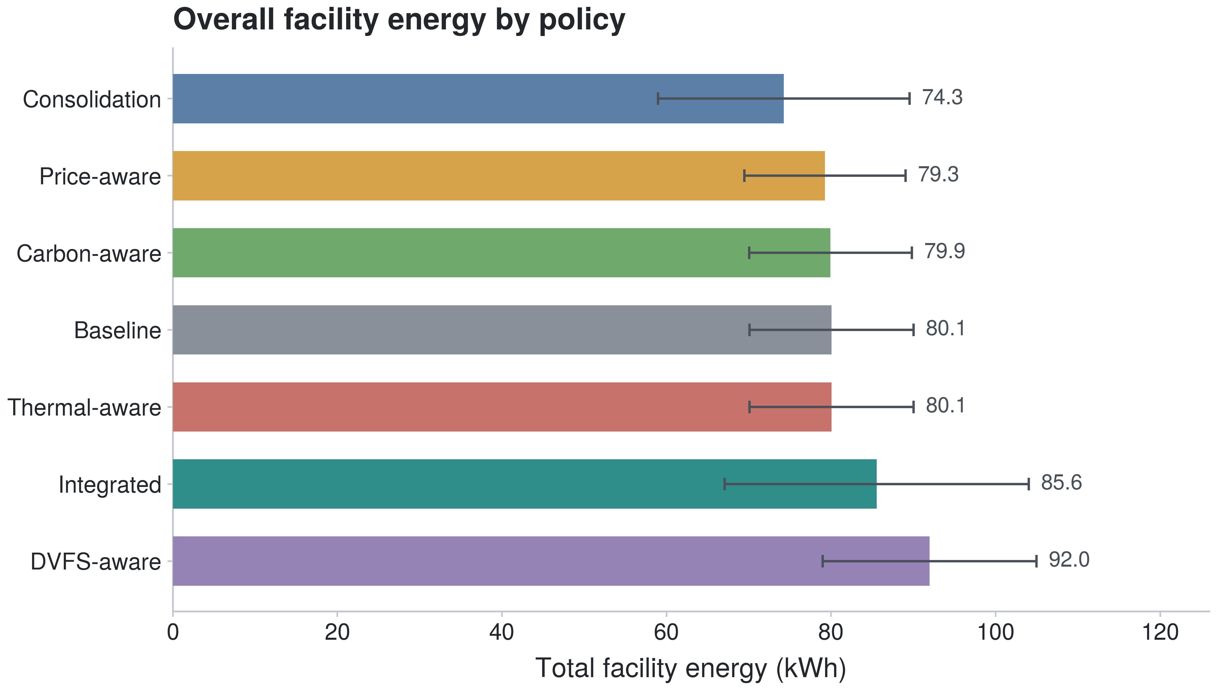
Figure 1. Total facility energy by policy, averaged across all scenarios and seeds. Lower is better.
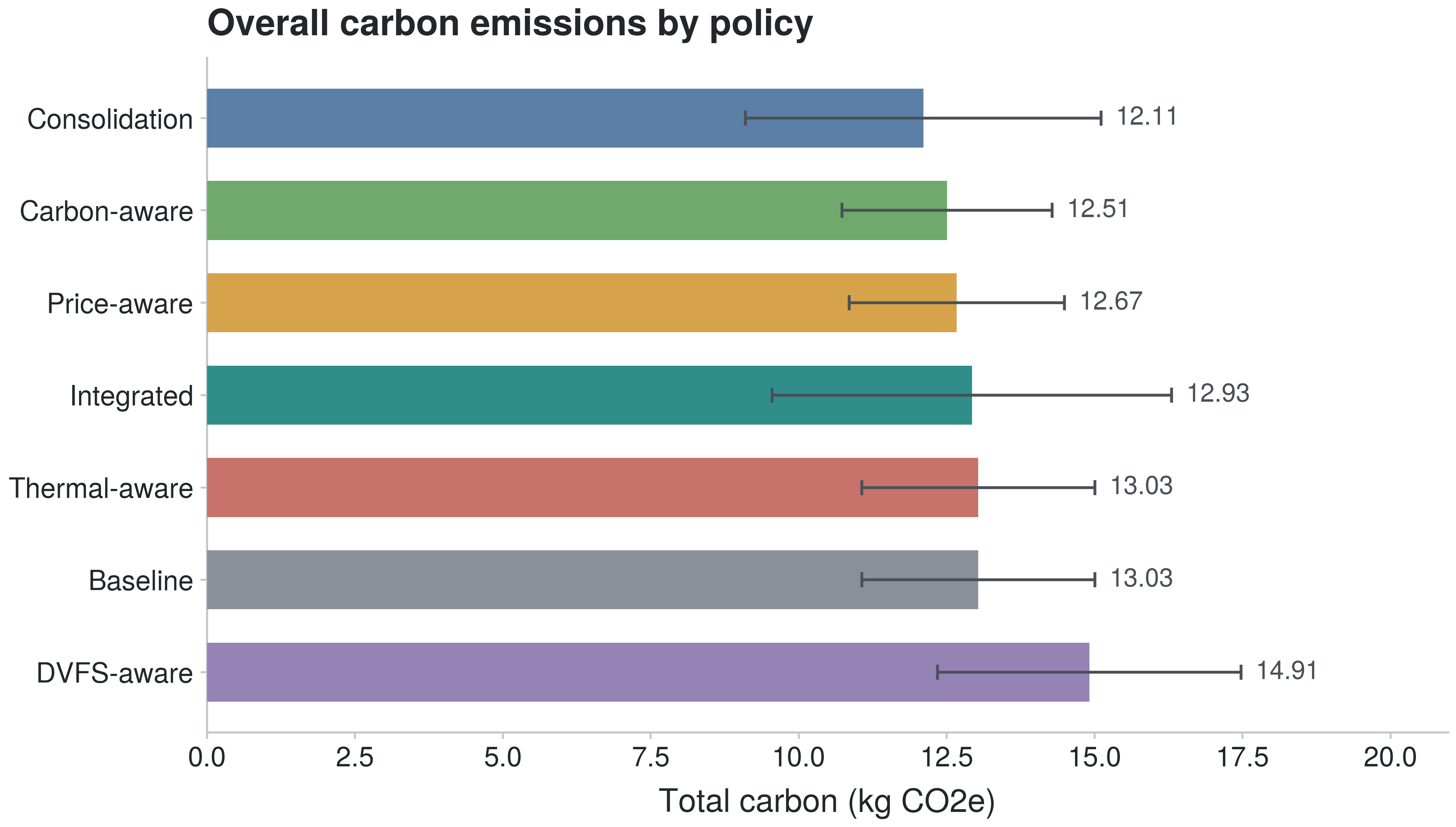
Figure 2. Total carbon emissions by policy, averaged across all scenarios and seeds. Lower is better.
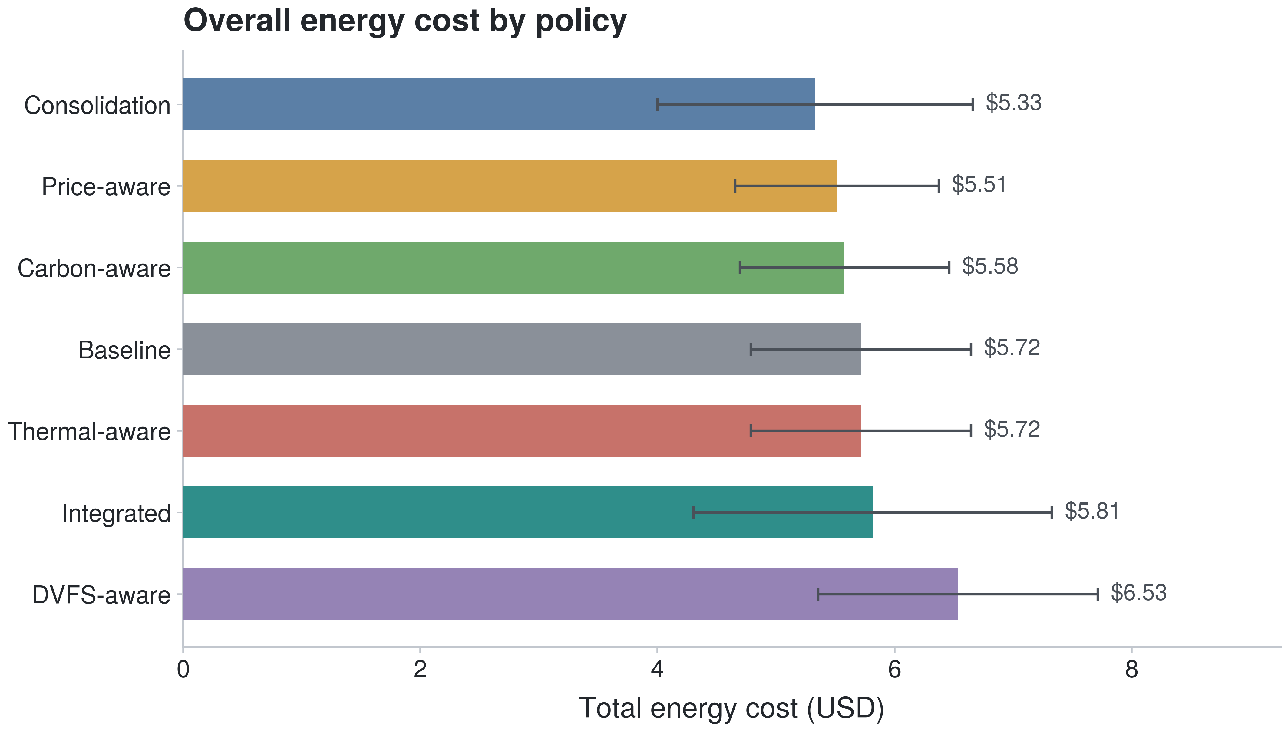
Figure 3. Total electricity cost by policy, averaged across all scenarios and seeds. Lower is better.
The three metrics move together, and consolidation sits at the low end of all of them while DVFS-aware sits at the high end of all of them. This alignment is the first substantive result. In this harness, the actions that reduce energy also reduce carbon and cost, because carbon and cost are computed from facility energy scaled by grid signals, so a policy that lowers kilowatt-hours generally lowers both derived quantities unless it deliberately shifts work in time. The exceptions are the carbon-aware and price-aware policies, which lower carbon and cost slightly more than they lower raw energy because they move flexible work toward cleaner or cheaper windows rather than simply using less power.
Figure 6 makes the point that average PUE is not where the differences live. Every policy sits near 1.32, and the spread between the best and worst is small enough that the figure has to be drawn as a divergence from baseline to be legible at all.
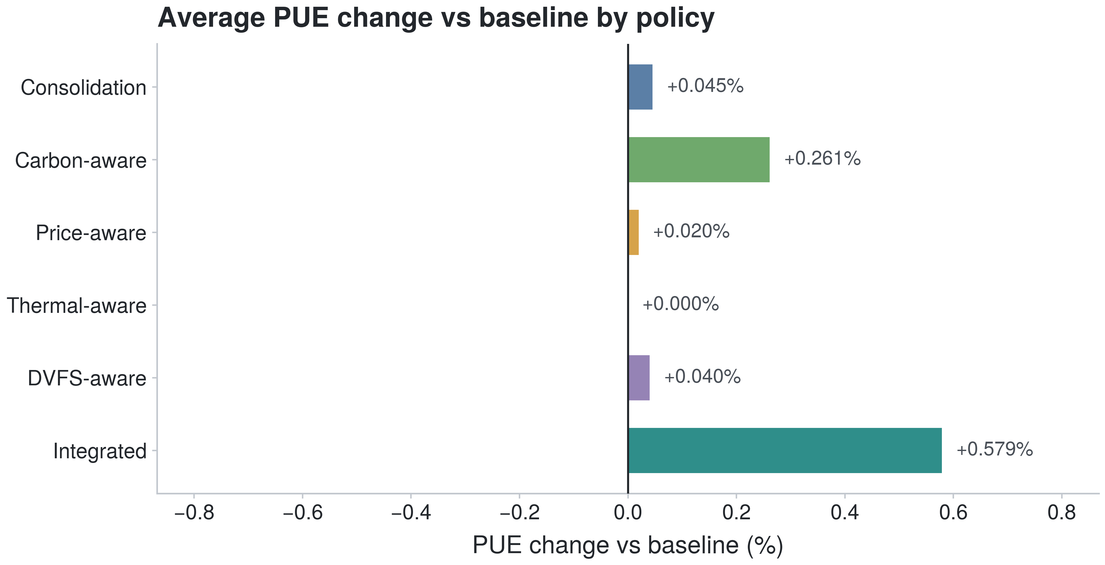
Figure 6. Average PUE expressed as percent difference from the baseline PUE, centered at zero. Negative is a lower, better PUE than baseline. Absolute differences are small because all policies operate near a PUE of 1.32.
That result is worth stating plainly, because PUE is the metric operators reach for most often. Under this reduced-order cooling model the policies barely separate on PUE, yet they separate clearly on total facility energy in Figure 1. The reason is that facility energy responds to how many servers are active and how hard they are driven, while PUE only measures the ratio of facility to IT power. A policy can hold PUE almost constant and still cut total energy by reducing IT load, which is exactly what consolidation does. This mirrors the caution in the cooling literature that PUE is a ratio rather than a measure of total consumption (Gao, n.d.).
Figure 7 collapses the aggregate story into relative change against the baseline for energy, carbon, and cost in a single view.
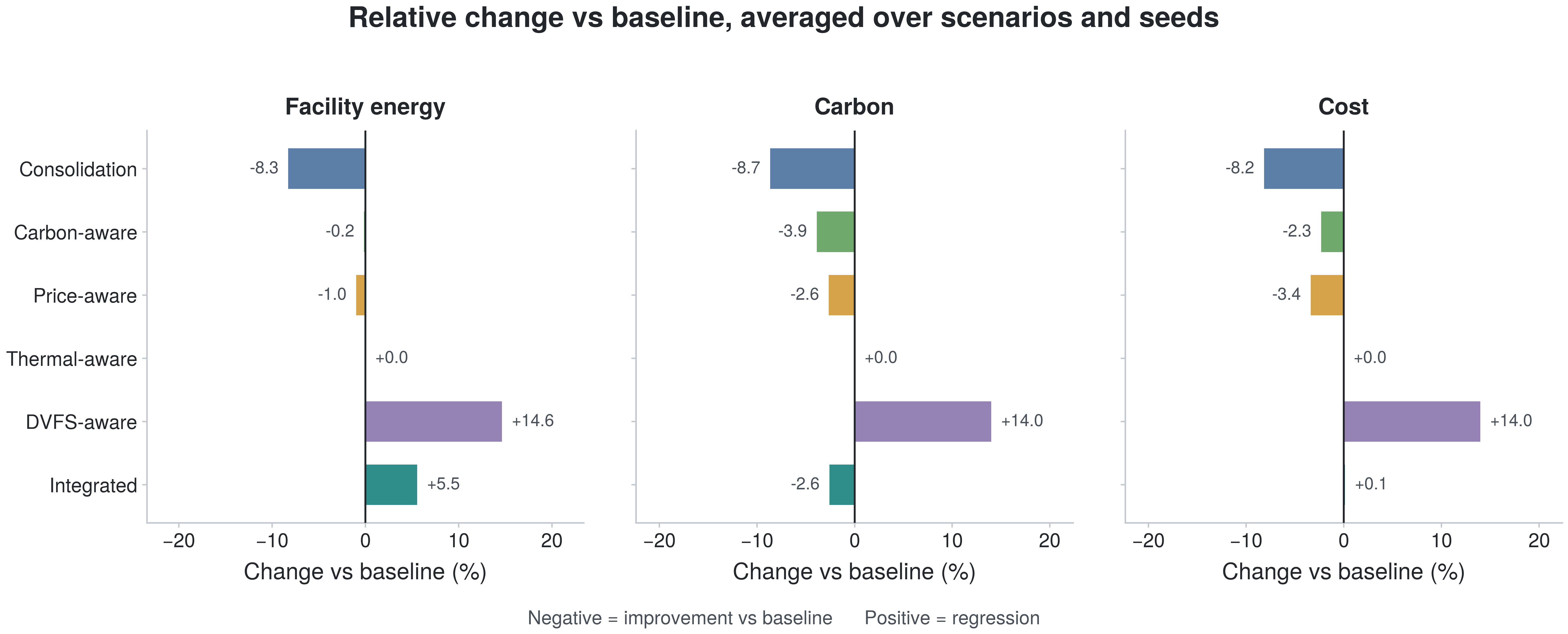
Figure 7. Relative change versus baseline for facility energy, carbon, and cost, averaged across scenarios and seeds. Negative values are improvements; positive values are regressions.
Consolidation delivers the largest reductions, near 8% on all three axes. Carbon-aware and price-aware produce smaller single-digit improvements, weighted toward the metric each targets. Thermal-aware is indistinguishable from baseline, a result explained in Section 7.3. Integrated coordination lowers carbon by about 3% and holds cost near baseline while raising facility energy by about 5%. DVFS-aware is the clear regression, adding roughly 14% to all three metrics. That the most hardware-focused single-objective policy is also the worst overall is the sweep’s most counterintuitive finding, and Section 8 takes it up directly.
7.3 Reliability and Thermal Tradeoffs
Energy, carbon, and cost do not capture whether a policy kept its promises to workloads. Figures 4 and 5 add the two constraint metrics that expose the cost of chasing efficiency: deadline misses and thermal violations.
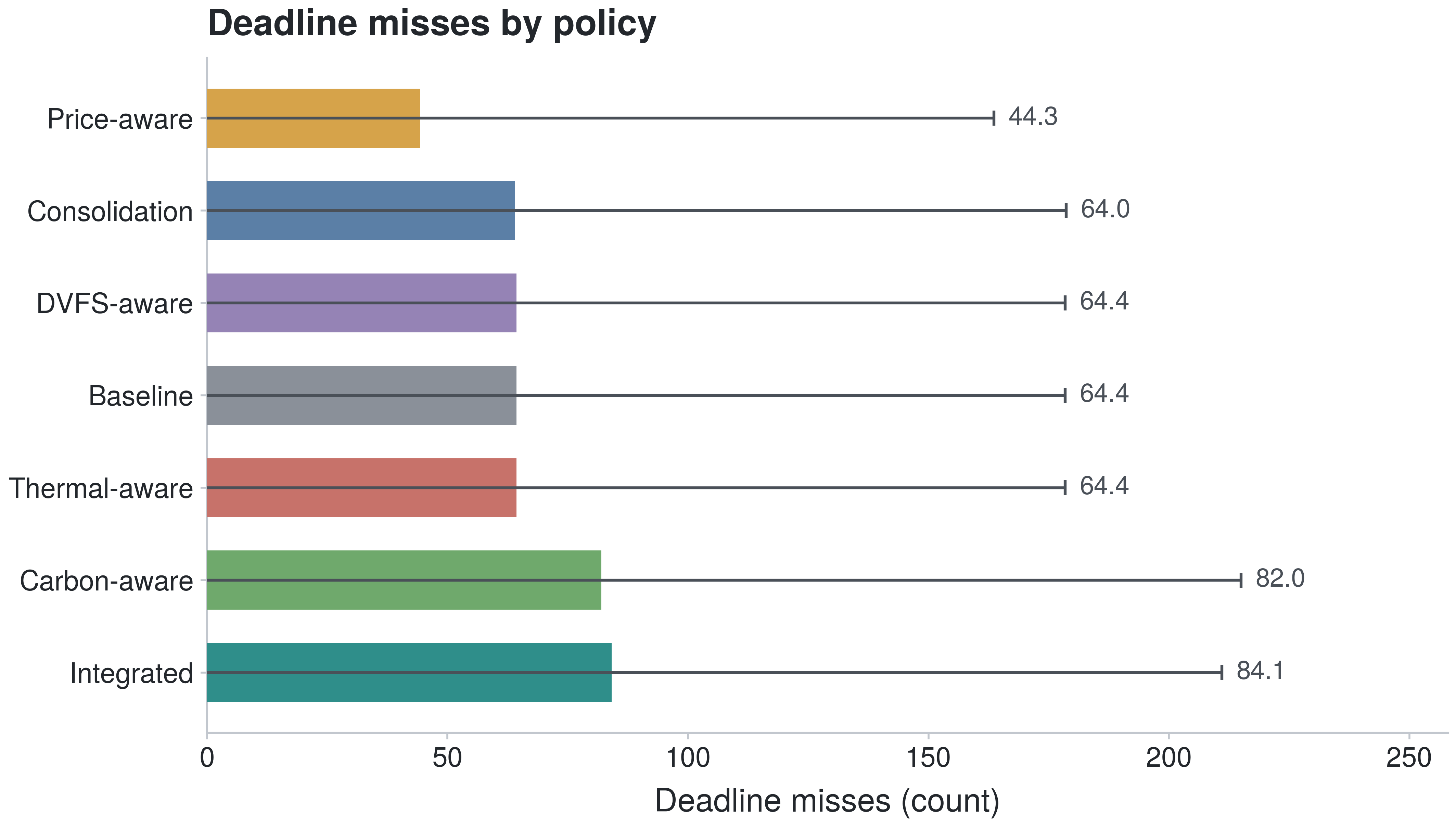
Figure 4. Deadline misses by policy, averaged across all scenarios and seeds. Lower is better.
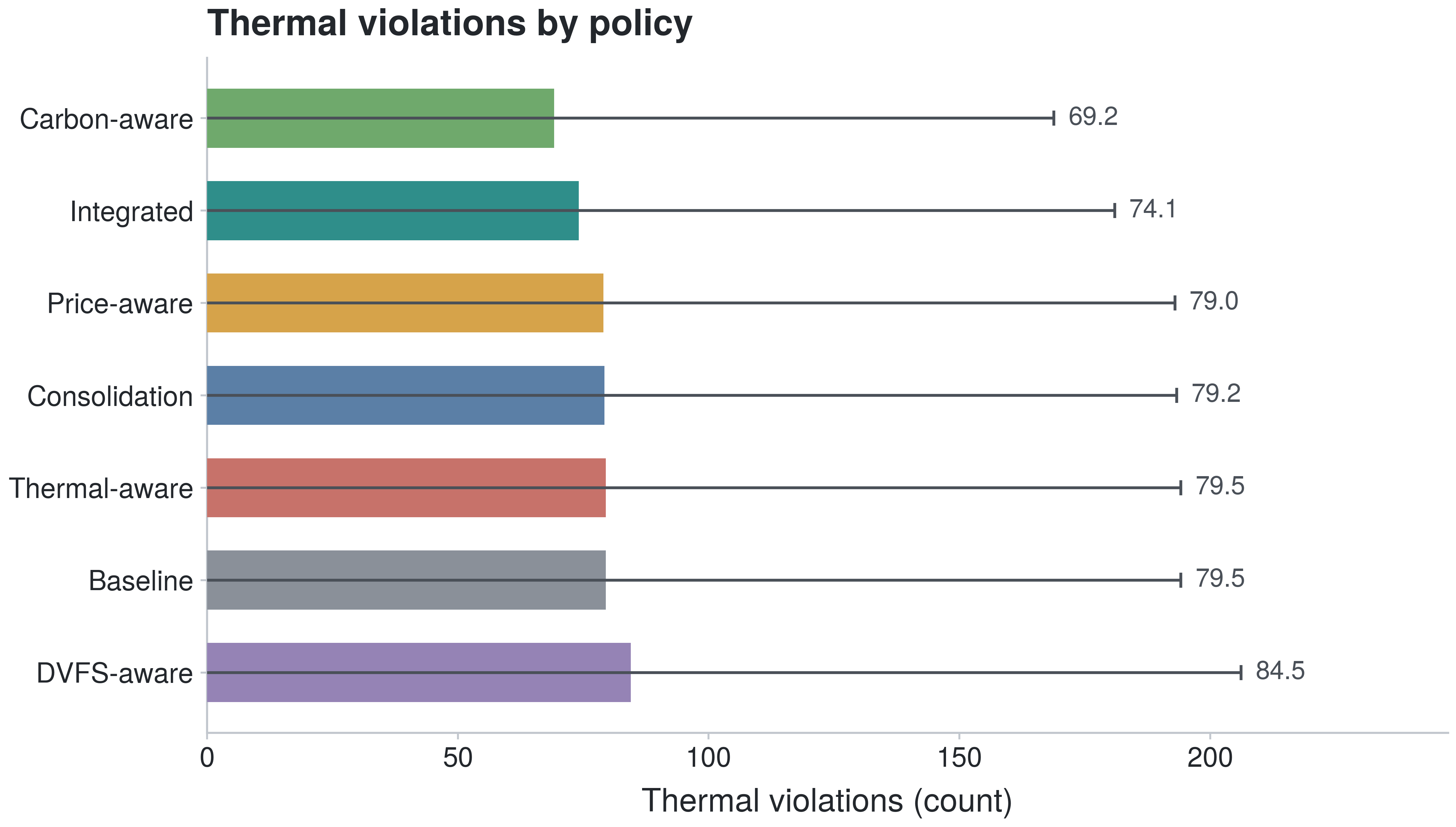
Figure 5. Thermal violations by policy, averaged across all scenarios and seeds. Lower is better.
The reliability picture inverts part of the efficiency picture. Price-aware records the fewest deadline misses, well below baseline, because deferring flexible work to cheaper windows in these scenarios also tended to relieve queue pressure at the moments that mattered for deadlines. Carbon-aware and integrated coordination go the other way and miss more deadlines than baseline. Both spend workload flexibility to reach cleaner grid windows or better-coordinated placements, and in a constrained fleet that deferral occasionally pushes a flexible job past its deadline. The integrated policy, which combines several such objectives, records the most deadline misses of any policy in the mean, though the seed-level variance on this metric is large enough (Table 3) that the ordering among the higher-miss policies should be treated as indicative rather than firm.
Thermal violations tell a complementary story. Carbon-aware and integrated coordination produce the fewest, while DVFS-aware produces the most. The thermal benefit of the carbon-aware and integrated policies is a side effect of moving work off the busiest servers during stressed periods, which lowers local heat generation. DVFS-aware raises thermal violations because holding servers in altered power states lengthens jobs and keeps hardware active and warm for longer. The single result that most complicates a simple reading is thermal-aware: it matches baseline exactly on every metric, including thermal violations. Under the reduced-order thermal model used here, the thermal-aware policy did not diverge from first-fit placement often enough to change outcomes, which says more about the fidelity of the harness than about the value of thermal-aware scheduling as a mechanism. Section 10 returns to this limitation.
Taken together, Figures 4 and 5 establish that no single-objective policy improves reliability and thermal safety at the same time as energy. Price-aware buys reliability, carbon-aware and integrated buy carbon and thermal headroom, and each pays for its gain somewhere else. This is the tradeoff structure the coordination framework predicts rather than an artifact to be optimized away.
7.4 Scenario Dependence
Averages hide the fact that policy rankings change with the operating regime. Figures 8 through 10 show the per-scenario deltas against baseline for energy, carbon, and cost as heatmaps, with scenarios on the rows and policies on the columns.
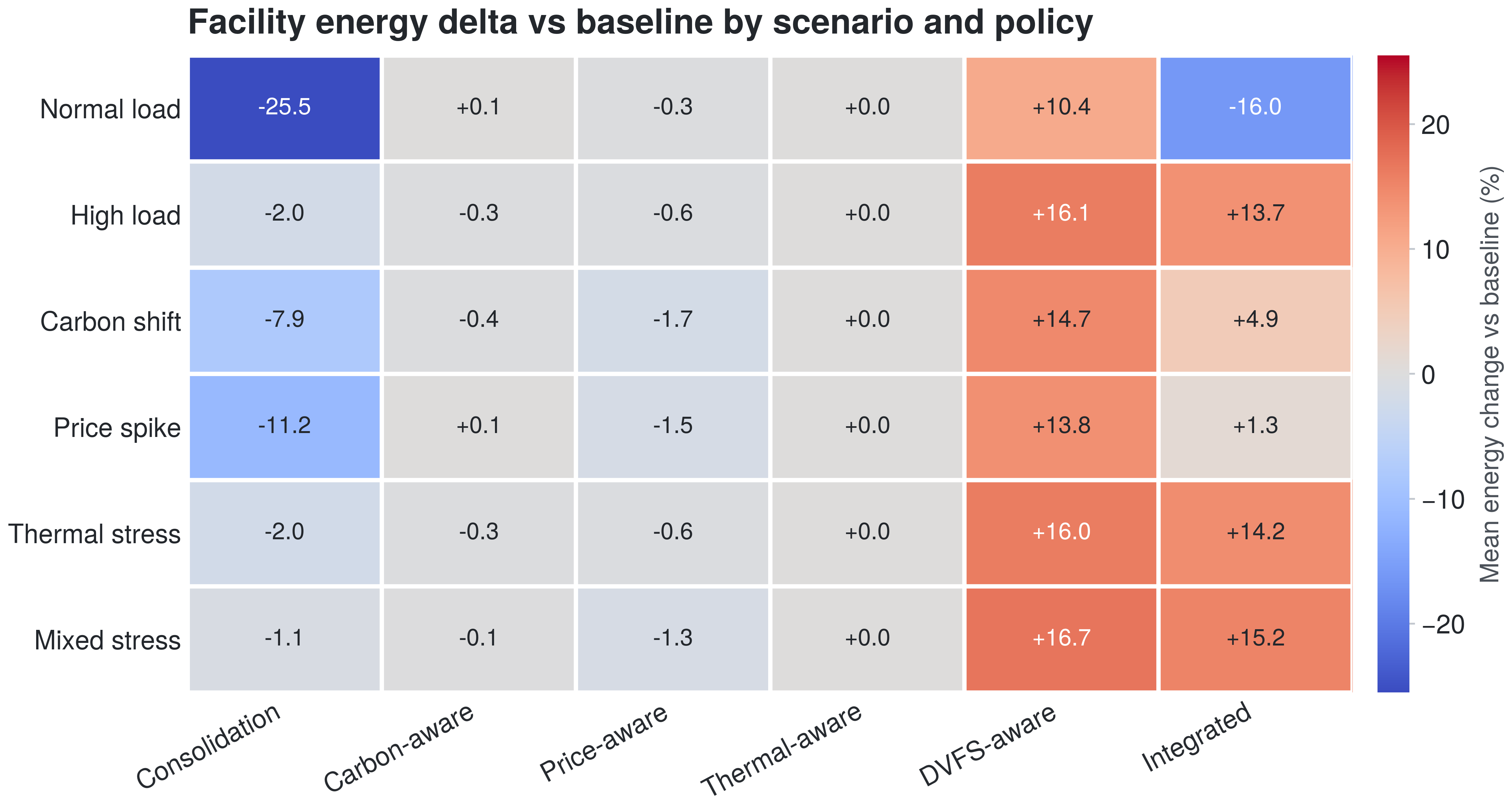
Figure 8. Facility energy change versus baseline by scenario and policy. Blue is a reduction; red is an increase.
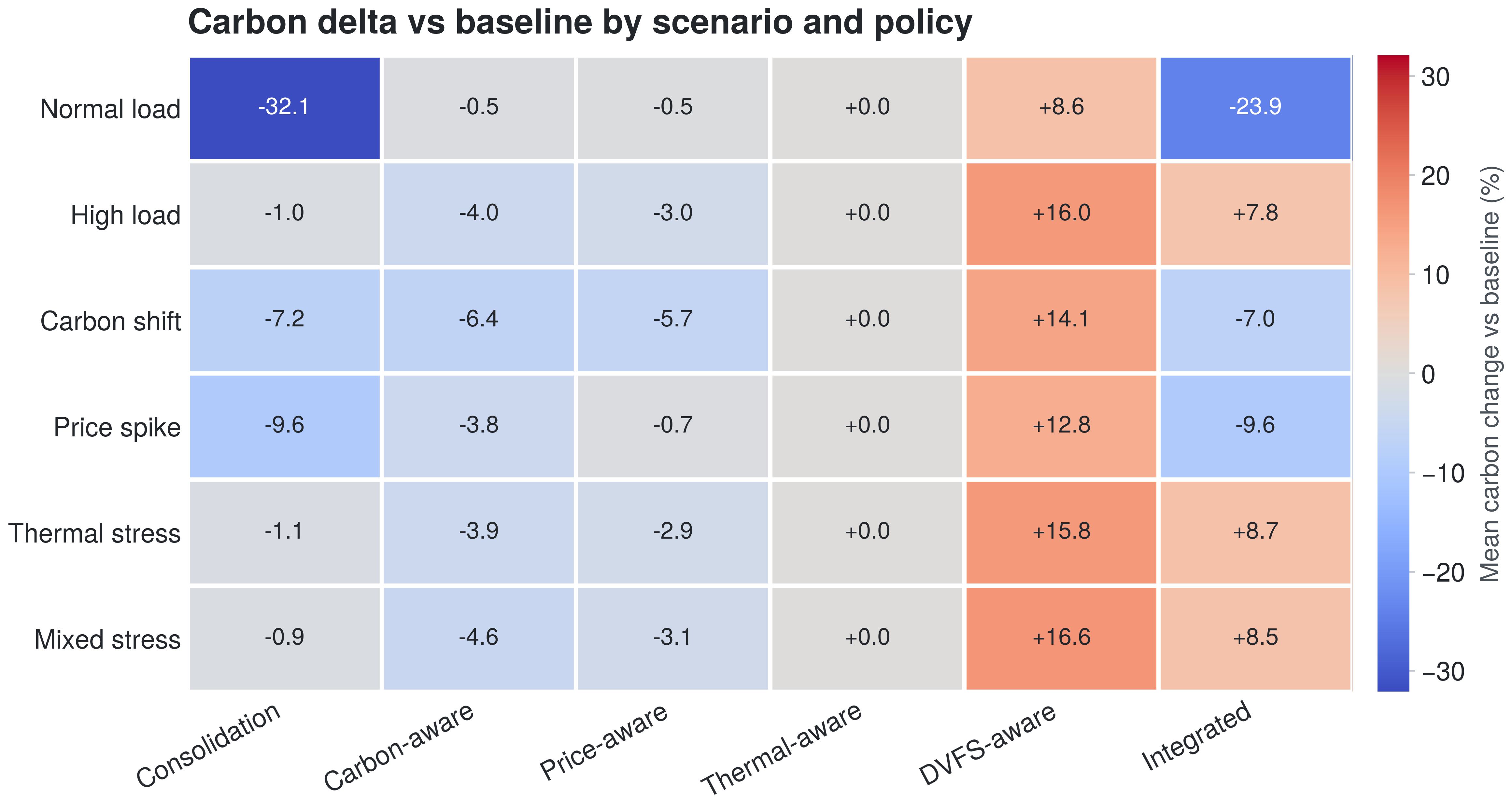
Figure 9. Carbon change versus baseline by scenario and policy. Blue is a reduction; red is an increase.
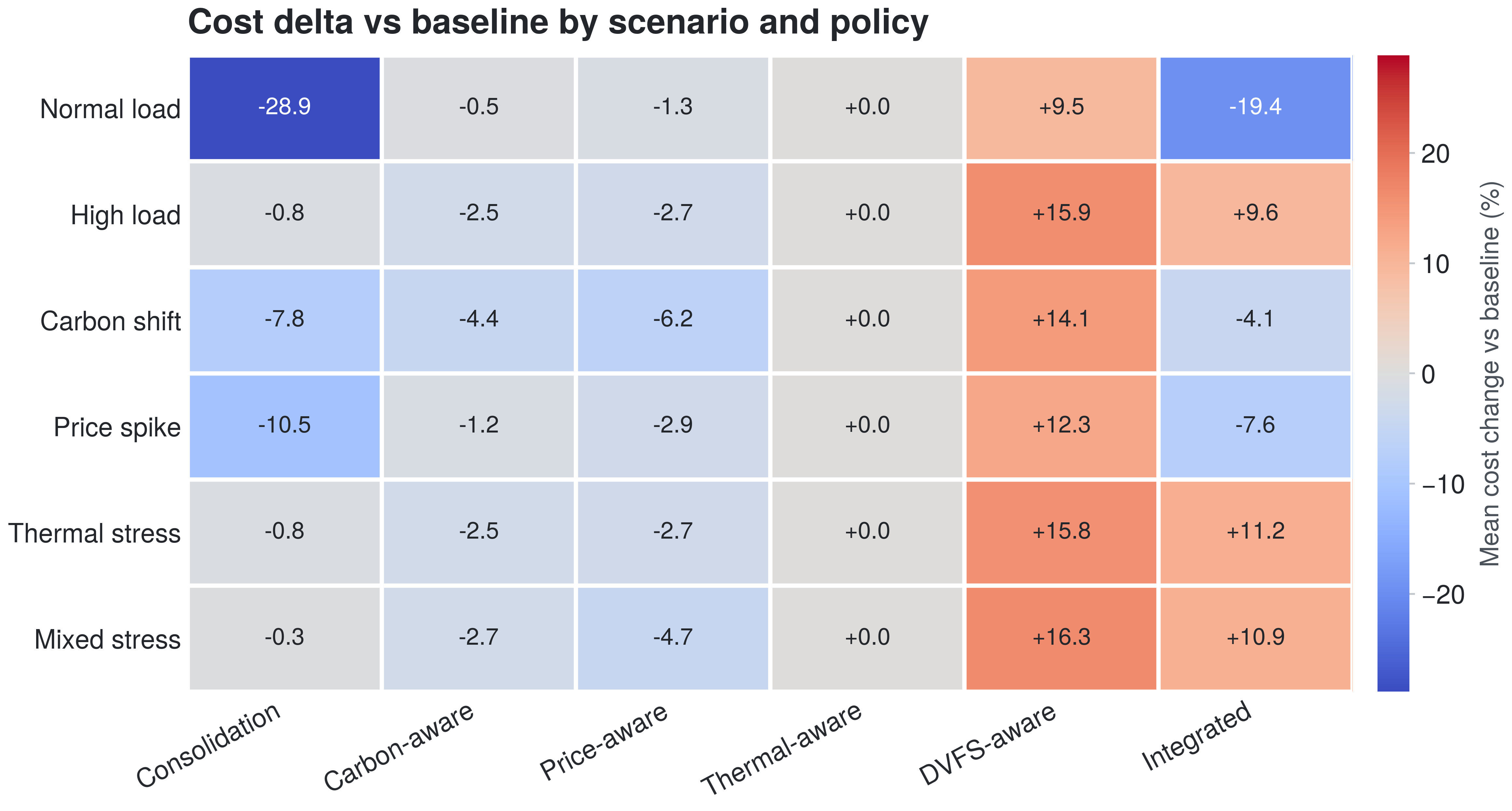
Figure 10. Cost change versus baseline by scenario and policy. Blue is a reduction; red is an increase.
The deepest blue cell in all three heatmaps is consolidation under the normal-load scenario, where it cuts facility energy from about 63 kWh to about 47 kWh, carbon from about 9.6 kg to about 6.6 kg, and cost by a comparable margin. That single scenario carries much of consolidation’s overall advantage. The mechanism is visible in the scenario energy bars of Figure 11.
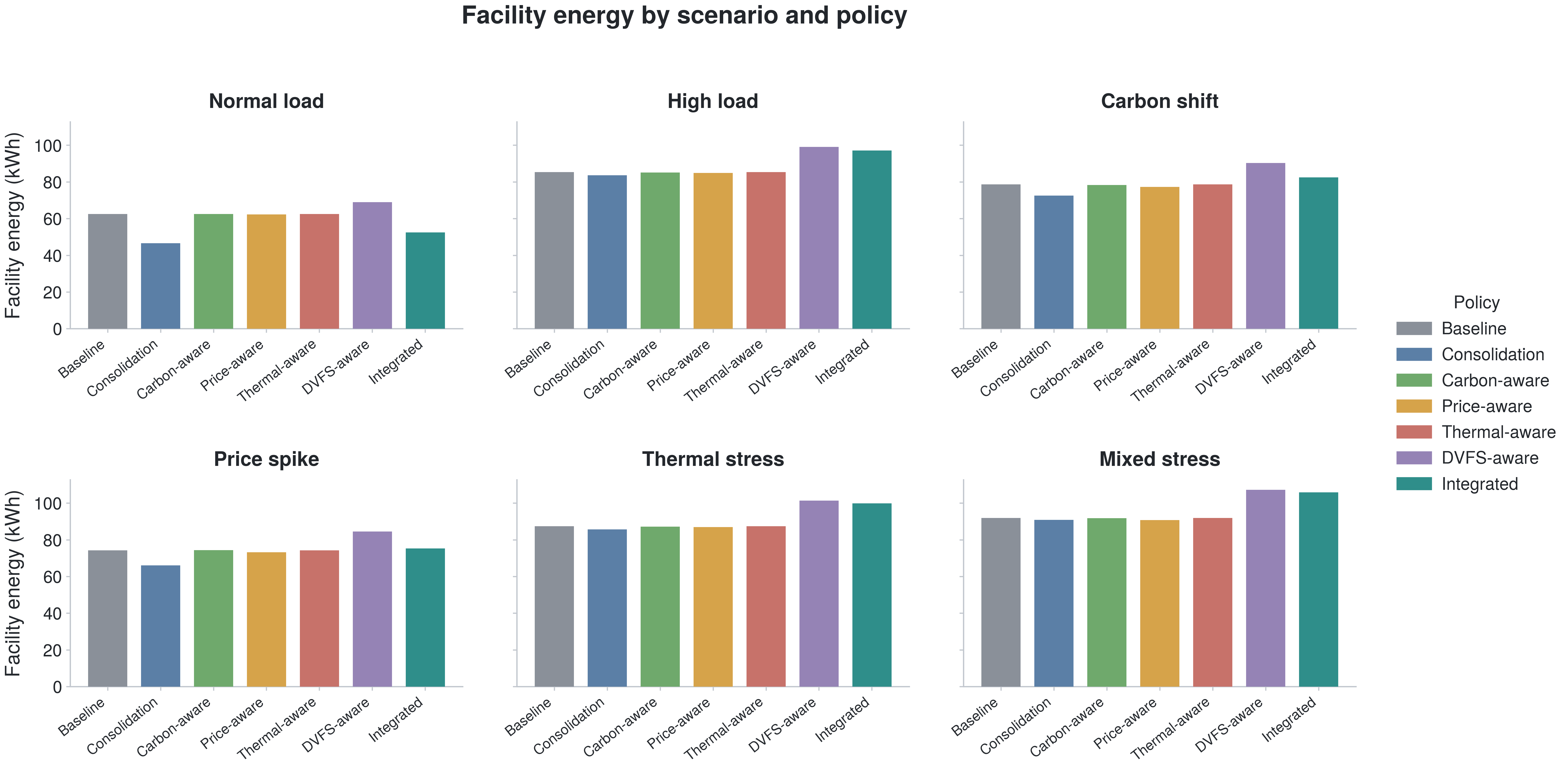
Figure 11. Facility energy by scenario and policy, one panel per scenario. Lower bars are better.
Under normal load there is slack to pack workloads onto fewer servers and sleep the rest, so consolidation and integrated coordination both pull well below baseline. Under high load and under the two stress scenarios the fleet is already busy, there are fewer idle servers to reclaim, and the consolidation advantage shrinks toward the baseline bar. The practical reading is that the largest efficiency lever in this study, reducing active server-hours, is available mainly when the fleet is underused, which is precisely when overprovisioning waste is largest.
Figures 12 and 13 show the same scenario breakdown for carbon and cost.
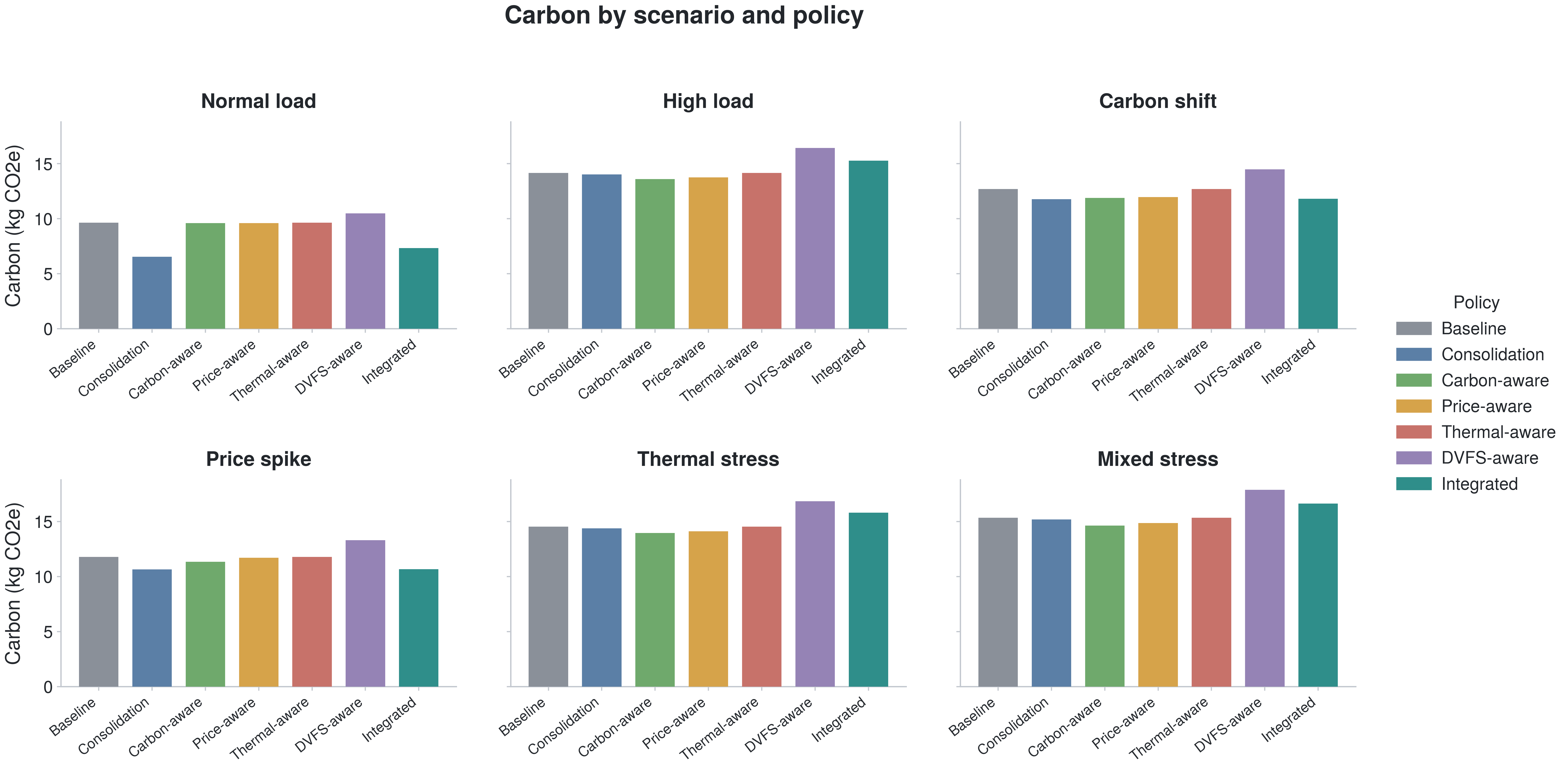
Figure 12. Carbon by scenario and policy, one panel per scenario. Lower bars are better.
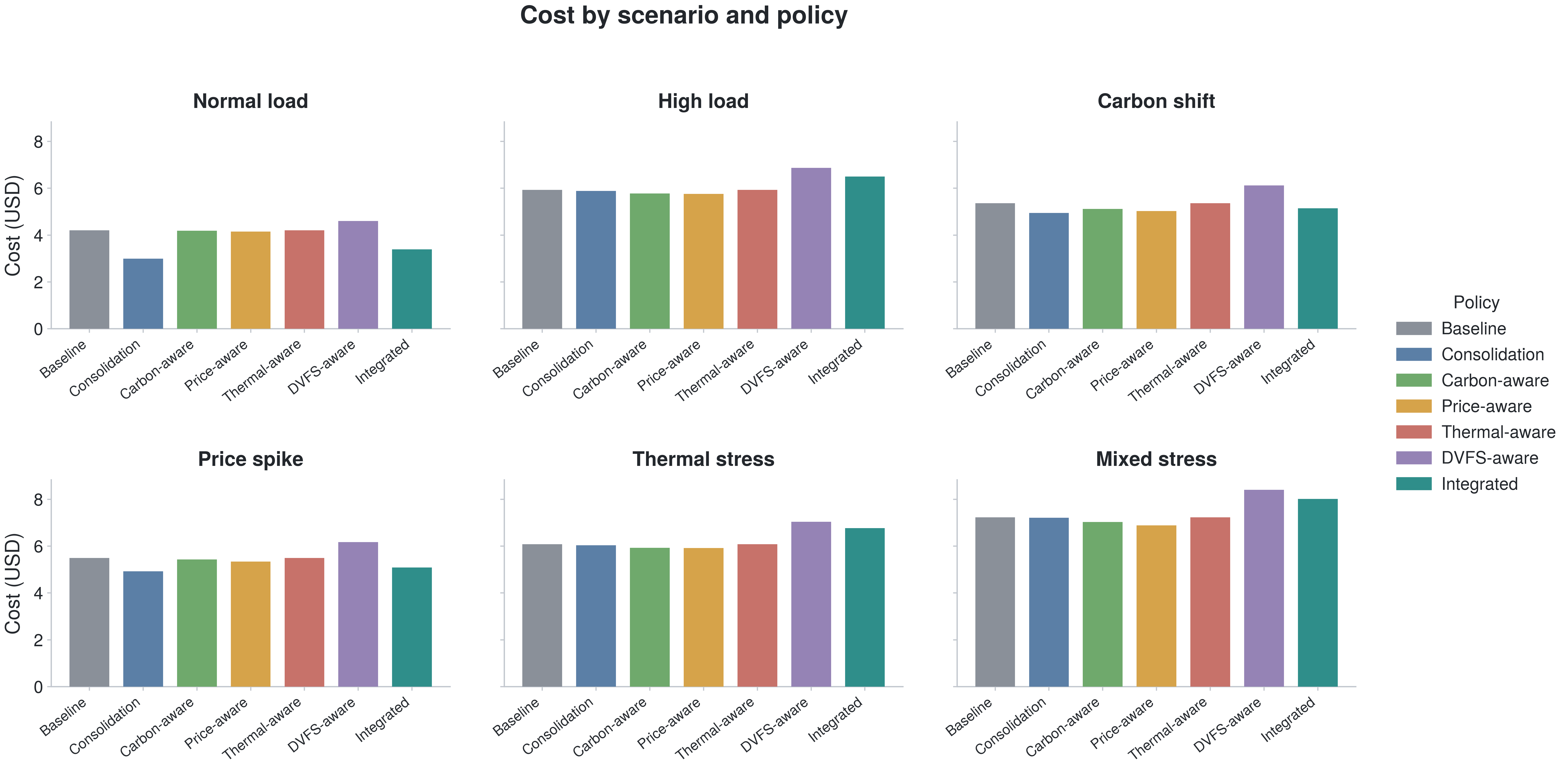
Figure 13. Cost by scenario and policy, one panel per scenario. Lower bars are better.
In the carbon-shift scenario, where flexible work can move into a cleaner grid window, consolidation, integrated coordination, and carbon-aware all reach the lowest carbon while DVFS-aware stays highest. During the price spike, consolidation and integrated coordination give the lowest cost, ahead of the price-aware policy that targets cost directly. That a general consolidation policy can beat the price-targeted policy on cost during a price spike is a useful reminder that the cheapest kilowatt-hour is often the one never drawn: reducing consumption competes with, and here slightly outperforms, timing consumption.
Thermal violations concentrate almost entirely in two scenarios, as Figure 14 shows.
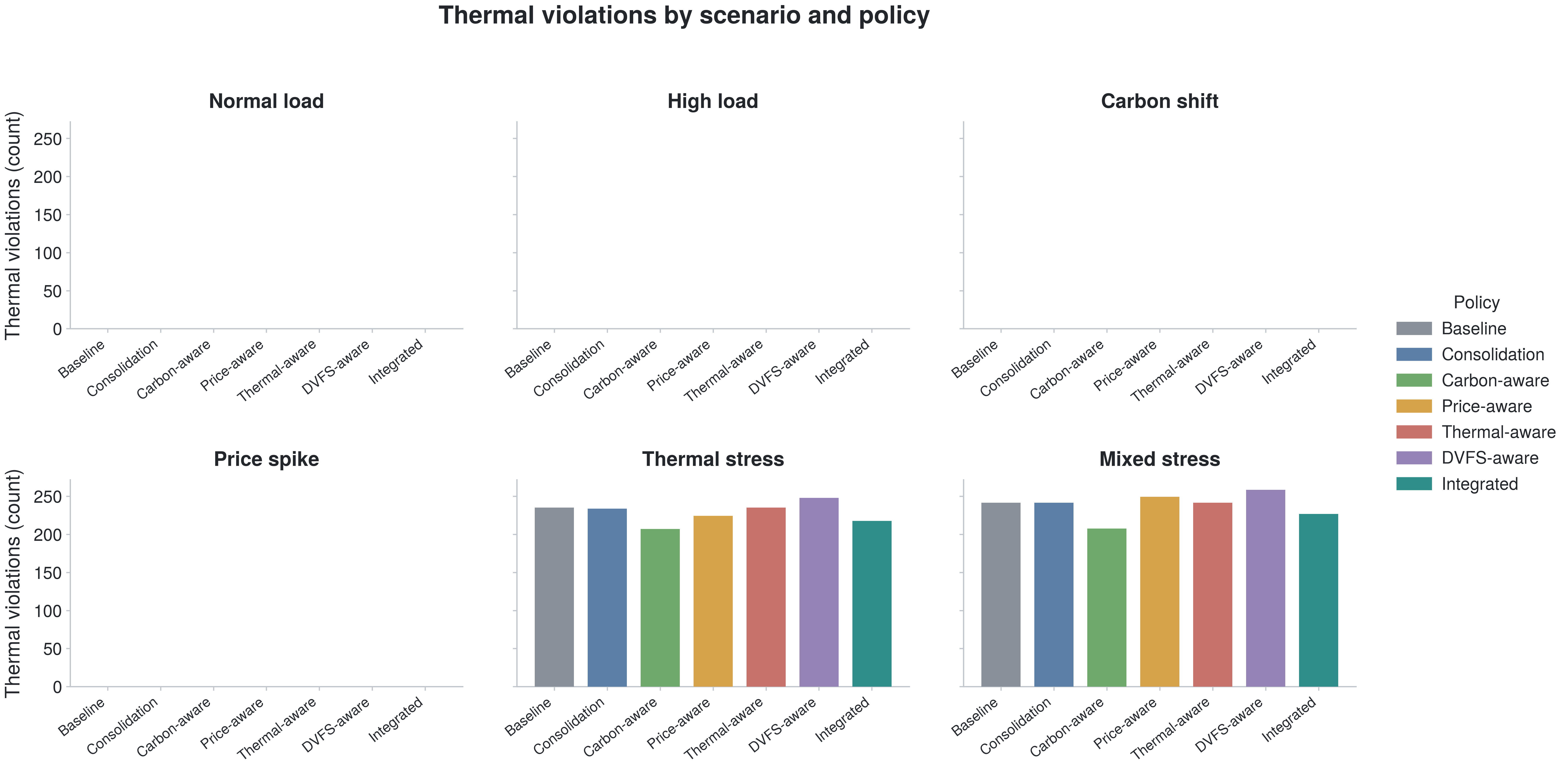
Figure 14. Thermal violations by scenario and policy, one panel per scenario. Lower bars are better.
Violations appear only under thermal stress and mixed stress. In both, carbon-aware and integrated coordination record the fewest and DVFS-aware the most, while thermal-aware again tracks the baseline rather than falling below it. The scenario view therefore reinforces the aggregate finding: the policies that help most under thermal stress are the ones that move work away from hot, busy servers, and the nominal thermal-aware policy is not among them under this harness.
7.5 Structural Relationships
Three scatter plots make the underlying relationships explicit and explain why the policies behave as they do. Figure 15 plots active server-hours against facility energy.
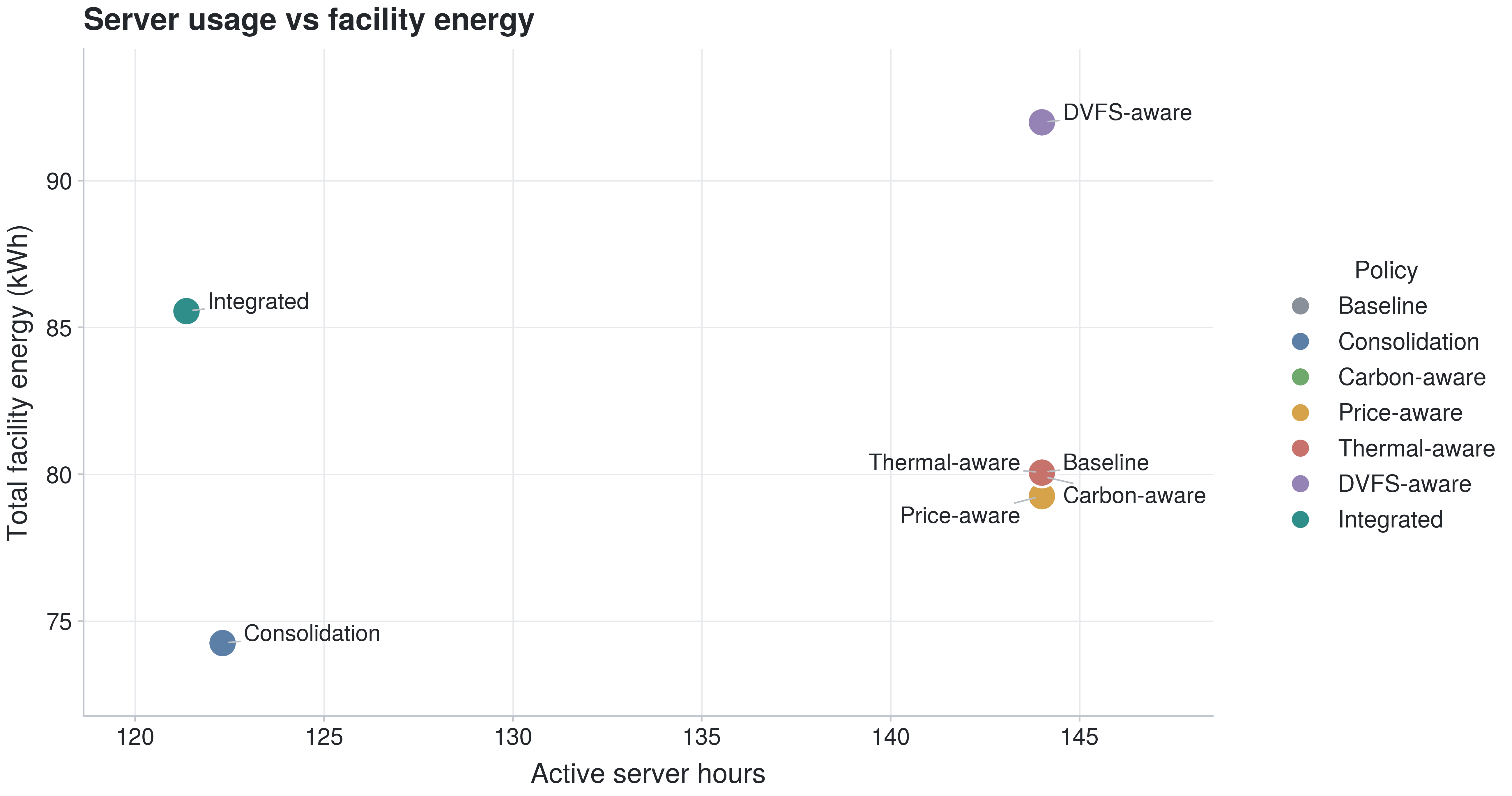
Figure 15. Active server-hours versus facility energy, one point per policy.
The points fall along a rising line, and consolidation and integrated coordination sit at the low-energy, low-server-hour end while the policies that leave all servers active cluster at the high end. This is the clearest single-variable explanation in the study: facility energy in this fleet is driven mostly by how many server-hours are kept active, and the policies that reduce active server-hours are the ones that reduce energy. It also explains why DVFS-aware regresses, since holding all 144 server-hours active while altering power states does nothing to reclaim idle capacity.
Figure 16 plots carbon against cost.
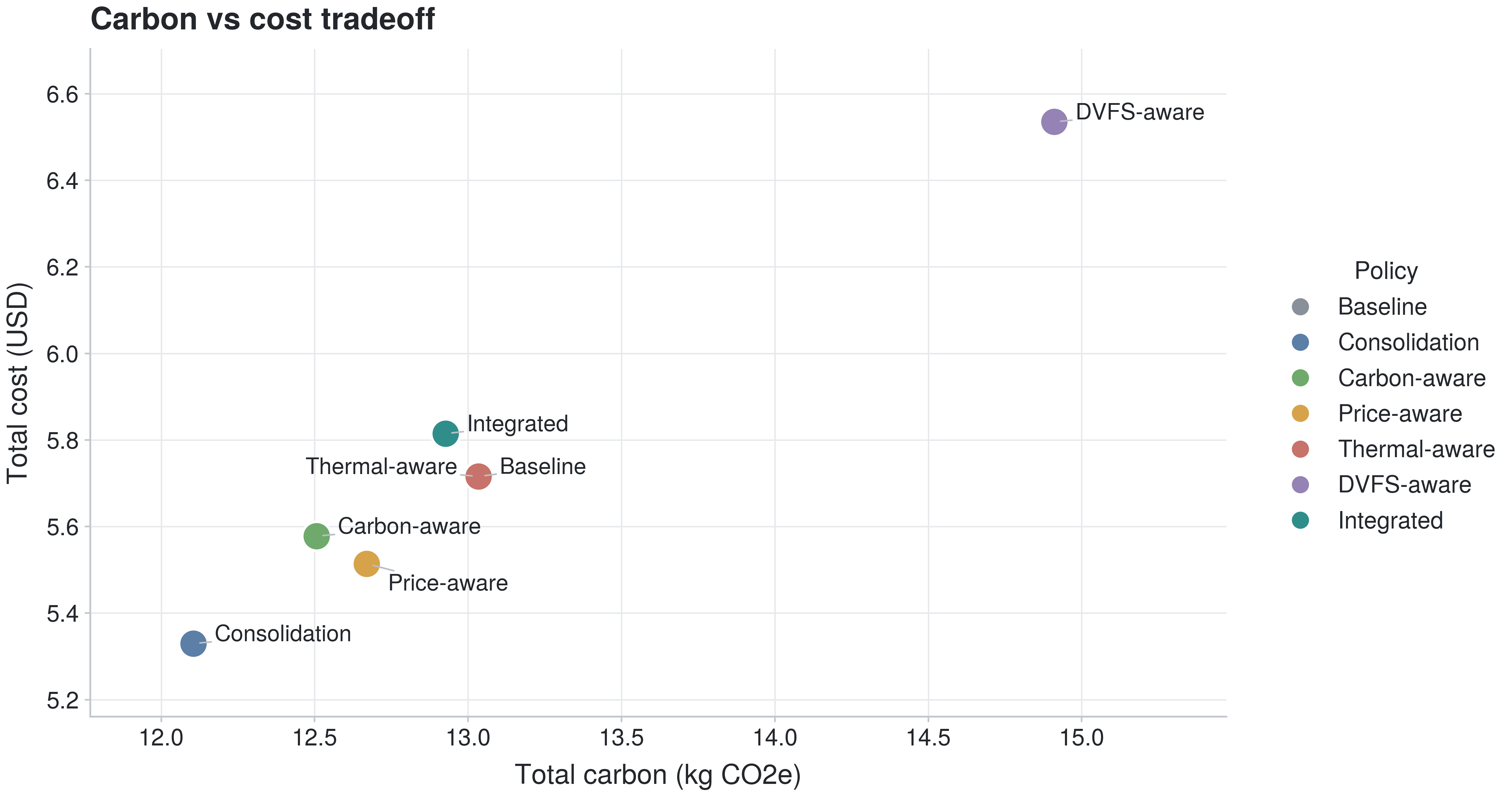
Figure 16. Total carbon versus total cost, one point per policy.
The two rise together rather than trading off. In these scenarios a policy that cuts carbon also cuts cost, because both are dominated by total energy and the grid signals did not diverge sharply enough to force a choice between clean and cheap. That will not hold in every real market, but within this sweep carbon and cost are complementary objectives, not competing ones.
Figure 17 plots the 95th-percentile rack temperature against deadline misses.
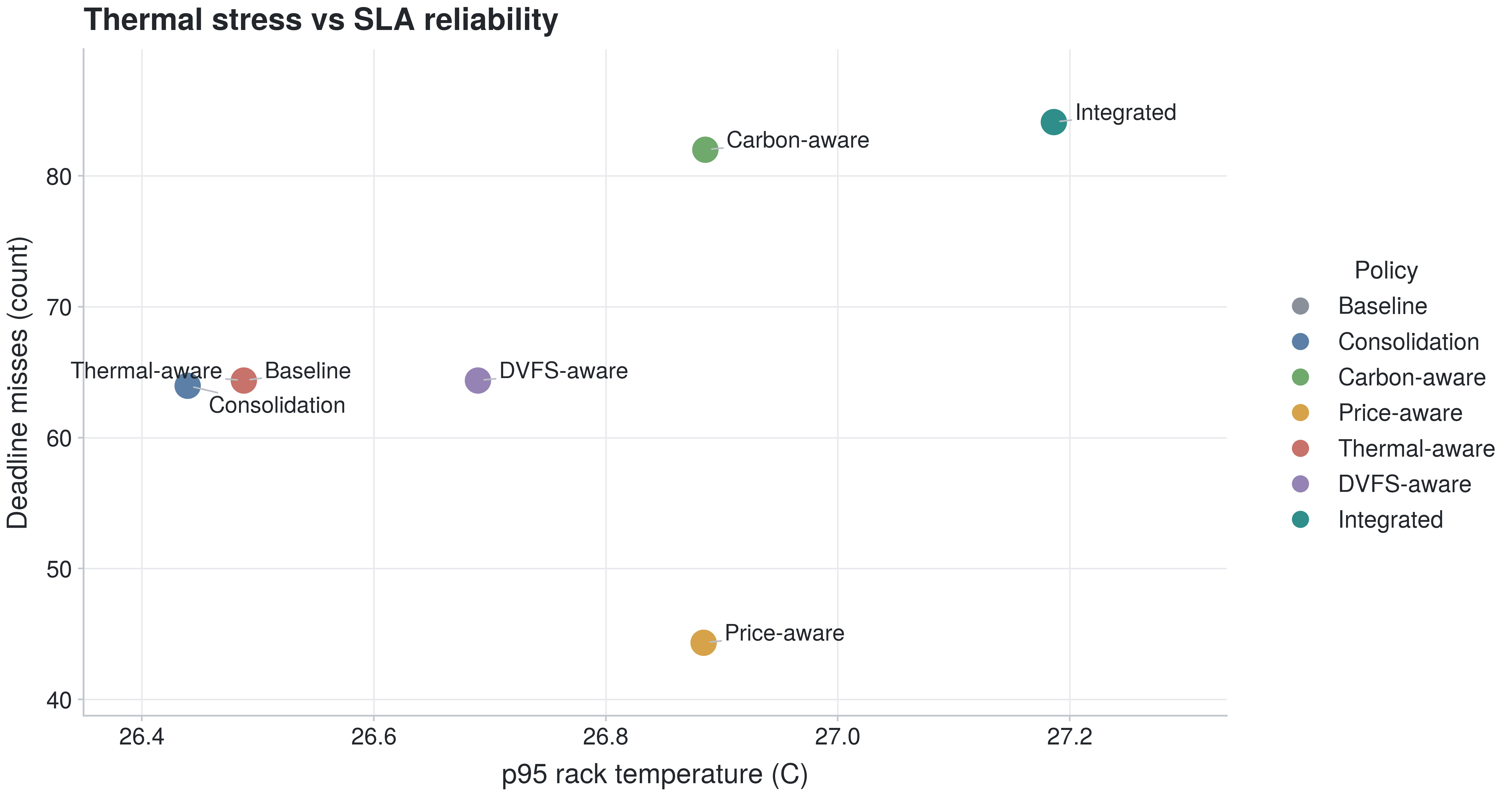
Figure 17. 95th-percentile rack temperature versus deadline misses, one point per policy.
Here there is no clean relationship. Higher rack temperature does not predict more deadline misses across policies, which means thermal stress and SLA risk are governed by different mechanisms in this model. A policy can run warm without missing deadlines, or miss deadlines without running warm, depending on whether its slack is spent on thermal relief or on chasing grid windows. The absence of a correlation is itself informative: it shows that thermal safety and deadline reliability have to be coordinated as separate constraints rather than assumed to rise and fall together.
Read as a whole, the comparative results support a single claim. Across seven policies and six scenarios, no policy dominates every metric, the largest efficiency gains come from reclaiming idle capacity rather than from any timing trick, and the policy that coordinates several objectives at once trades raw energy for lower carbon and better thermal safety instead of winning on all fronts. That is the behavior a coordination layer should show, and it sets up the interpretation that follows.
8. Discussion
The comparative results are modest in magnitude and specific in shape, and both properties matter for what they say about coordinated infrastructure control. The headline numbers are single-digit to low-double-digit percentage changes, not the large savings sometimes reported for production cooling deployments. That gap is expected, because this study evaluates scheduling and coordination policies inside a reduced-order simulator rather than tuning a real cooling plant, and the point of the sweep is the structure of the tradeoffs rather than any single savings figure.
The strongest and simplest finding is that reducing active server-hours does more for facility energy than any other single mechanism tested. Consolidation produced the largest reductions in energy, carbon, and cost, and Figure 15 shows why: energy tracks active server-hours almost linearly, so a policy that empties and sleeps underused servers reclaims power that idle-but-active machines would otherwise burn. This is consistent with the long-standing observation that servers draw a large fraction of peak power even when lightly used, and that consolidation is among the most reliable levers for energy efficiency in oversubscribed data centers (Ilager & Buyya, 2024; Farahnakian et al., 2014). The scenario breakdown adds a qualification that the aggregate hides. Consolidation’s advantage was concentrated under normal load and shrank under high load and stress, because a busy fleet offers little idle capacity to reclaim. The lever is real, but its size depends on how overprovisioned the fleet is at the moment, which is an argument for detecting the operating regime before choosing a policy rather than committing to one policy in advance.
The DVFS-aware regression deserves attention precisely because it runs against intuition. Dynamic voltage and frequency scaling is a well-established energy-saving mechanism, yet applied on its own in this sweep it raised energy, carbon, and cost by roughly 14% and produced the most thermal violations. The explanation is coordination, or its absence. DVFS reduces instantaneous power but can lengthen execution, and a job that runs longer keeps its server active and warm for longer, which in a model where energy tracks active server-hours can raise total energy even as instantaneous power falls. The DVFS literature is explicit that the mechanism trades power against performance and that it should be coordinated with placement and consolidation rather than applied in isolation (Liu, 2024; Arroba et al., 2017; Mazumder, 2022). The result here is a concrete instance of that warning: an isolated power-state policy, blind to placement and to how long its slowed jobs keep servers alive, moved the fleet in the wrong direction on every headline metric. Coordination is not a refinement of DVFS in this case; it is the difference between DVFS helping and hurting.
Carbon-aware and price-aware behavior confirms that timing flexibility is a genuine but bounded lever. Each policy improved its target metric by a few percent by moving deferrable work into cleaner or cheaper windows, which is the mechanism at the center of renewable-aware and market-aware scheduling research (Li et al., 2025; Jayanetti et al., 2024; Venkataswamy & Grimshaw, n.d.; Bahi et al., 2026). The cost of that flexibility showed up in reliability. Carbon-aware missed more deadlines than baseline, and the integrated policy, which layers several deferral objectives together, missed the most. This is the same tension those papers navigate when they add SLA terms to their reward functions, and it appeared here without being designed in: whenever a policy spends workload flexibility to chase a grid signal, some of that flexibility comes out of the deadline budget. A coordination layer does not remove this tension. It makes the tension explicit and lets an operator decide how much reliability to spend on carbon or cost.
The integrated coordination policy is the clearest test of the paper’s thesis, and its results are deliberately unglamorous. It lowered carbon by about 3% and held cost near baseline while raising facility energy by about 5% and missing more deadlines than any other policy. It did not dominate. What it did was move the operating point: it bought lower carbon and better thermal safety with higher energy and lower deadline reliability. Under a multi-objective scoring function that is exactly the expected behavior, because coordinating competing objectives reshuffles where costs land rather than eliminating them. The finding validates the framing that energy, carbon, thermal stability, and reliability are coupled outcomes of one coordinated system rather than independent targets, and it cautions against reading any integrated controller as a source of free savings. The honest description of coordination here is that it manages tradeoffs, and its value depends on whether the operator agrees with the tradeoff it chose.
The scenario dependence seen across Figures 11 through 14 supports the hierarchical view of infrastructure that the paper set out. The best policy changed with the regime: consolidation under normal load, price-aware for reliability under high load, carbon-aware and integrated under thermal stress. A fixed policy cannot be right in all of these, which is the case for a detection-driven layer that first identifies the binding constraint and then selects a coordinated response, rather than a single controller applied everywhere. This is the same conclusion the survey literature reaches when it argues that computing and cooling, and by extension workload and grid, must be managed together rather than as isolated subsystems (Ilager & Buyya, 2021; Rostami et al., 2023).
One result should be read as a limitation of the harness rather than a finding about mechanisms. The thermal-aware policy was indistinguishable from baseline on every metric. Under the reduced-order thermal model, thermal-aware placement did not diverge from first-fit often enough to matter, which contrasts sharply with the strong cooling results reported from higher-fidelity models and real deployments (Gao, n.d.; Zhou et al., 2024; Naug et al., 2024; Jadhav & Liu, 2026). The gap is a property of the simulator, not evidence against thermal-aware scheduling. It marks the boundary of what this study can claim and points directly at the fidelity improvements taken up in Section 10.
9. Practical Deployment and Operational Implications
9.1 A Phased Deployment Path
Nothing in these results argues for handing a data center to an autonomous controller. The coordination layer is better introduced in stages, each earning the trust the next one needs. The first phase is read-only monitoring and simulation: the system ingests workload, power, carbon, and weather signals, estimates the energy, thermal, and reliability consequences of current operations, and replays proposed policies in the simulator without touching production. Its value here is observability and a safe testbed, and it surfaces the fidelity gaps described in Section 10 before any action depends on them.
The second phase is operator-facing recommendation. The layer surfaces the binding constraint it detects, ranks candidate actions with the score breakdown of Section 6.4, and shows the predicted tradeoff, while an operator decides whether to act. This is where the paper’s honest treatment of tradeoffs pays off: an operator who can see that a proposed placement buys lower carbon at the cost of a deadline makes that call deliberately rather than discovering it afterward.
The third phase is guardrailed automation for low-risk actions. A narrow set of reversible, low-consequence decisions, such as sleeping a clearly idle server, deferring a batch job with ample slack, or nudging a cooling setpoint within a safe band, can be automated behind hard constraints and automatic rollback, while high-consequence actions stay with the operator. The fourth phase is closed-loop learning from approved actions and verified outcomes. Once the recommendation and guardrail phases have produced a log of human-vetted decisions and their measured results, that log becomes training data for the learned policies discussed in Section 10, closing the loop from detection through coordination and local optimization to verification.
9.2 Where Near-Term Value Is Most Likely
The near-term value of this work is most likely in decision support rather than autonomous control, and it is not evenly distributed. The operators with the most to gain are those without hyperscaler-scale internal optimization teams: GPU cloud providers, HPC centers, enterprise AI clusters, colocation operators, and regional data center operators. Hyperscalers already run sophisticated in-house schedulers and cooling controllers, so the marginal value of an external coordination layer is smaller for them. For everyone else, a system that detects the binding constraint, explains the tradeoff, and verifies the outcome offers a route to better coordination without building that capability from scratch.
9.3 Return on Investment
The commercial case follows the same discipline as the technical one and should not be overstated. A first-order estimate of annual savings is
Annual savings = annual energy spend × achievable percentage reduction under the applicable operating regimes
The two factors are not independent of the results above. The achievable percentage is regime-dependent. The sweep suggests the largest savings appear when underutilized capacity can be consolidated, which is exactly the normal-load regime where idle server-hours are available to reclaim, and that the margin shrinks toward zero on a fleet that is already busy. A chronically overprovisioned facility has the most to gain; one that already runs hot has little consolidation headroom, and coordination there would act mainly on carbon and thermal risk rather than on the energy bill. Because the percentage is both regime-dependent and, in this study, simulated, any figure carried into a business case has to come from site-specific validation on the operator’s own workloads and grid signals rather than from the numbers reported here.
10. Limitations and Future Work
It is worth stating the study’s limitations together before turning to future work, because several of them bound the results in ways that matter. The main ones are the reduced-order thermal and cooling model; synthetic or weak SLA and deadline labels; the absence of real facility telemetry; a heuristic fixed-weight coordination policy rather than a learned one; limited regional modeling that under-exercises the fleet layer; no validation on real hardware; a possible mismatch between public traces and the AI production workloads the framework targets; the lack of real operator-behavior data to calibrate the recommendation and approval loop; and limited modeling of network transfer, live migration, data locality, and regulatory or compliance constraints on where work may run. The paragraphs that follow take up the most consequential of these in turn.
The central limitation is fidelity. The simulator uses reduced-order models for power, cooling, and rack temperature, and it does not represent airflow, chilled-water loops, heat recirculation, or the slow dynamics of real cooling plants. The clearest symptom is the thermal-aware policy collapsing onto the baseline, which shows that the thermal model is too coarse to reward good placement. Higher-fidelity thermal modeling, whether through calibrated physical simulators of the kind used in recent cooling work or through validated surrogates, is the most important next step, because several of the mechanisms this paper reviews only pay off when the thermal consequences of placement are modeled accurately (Rostami et al., 2023; Zhou et al., 2024; Jadhav & Liu, 2026).
A second limitation is that the integrated coordination policy is a heuristic multi-objective function with fixed weights, not a learned controller. It applies the scoring function of Section 6.4 with static coefficients, so it cannot adapt its tradeoffs to the regime it detects, and its deadline-miss penalty was evidently too weak relative to its carbon and thermal terms. Replacing the fixed weights with a policy learned from simulator rollouts is the natural progression. Offline reinforcement learning is a promising route because it can learn from logged experience without exploring unsafe actions on a live fleet, an approach that has produced safe cooling controllers elsewhere (Zhou et al., 2024). For coordination across regions and facilities, multi-agent reinforcement learning is the closest existing family of methods, though its known problems with non-stationarity, partial observability, and scalability would have to be addressed before it could drive real fleets (Jayanetti et al., 2024; Yao et al., 2022; Hady et al., 2025).
The evaluation also leans on weak labels for the properties the control problem most needs. Public traces rarely record deadlines, SLA tolerances, or migratability, so these were inferred from workload type or assigned synthetically. The deadline-miss results in particular depend on those assumptions, and a policy tuned against synthetic deadlines may behave differently against real ones. Future work should test the sensitivity of the reliability results to the labeling rules and, where possible, validate them against traces that carry genuine SLA information.
The fleet abstraction used in these runs under-exercises the regional layer that the framework places above facility control. The scenarios varied load and grid signals but did not model a true multi-region fleet with distinct capacities, network costs, and carbon profiles, which is where the argument for cross-region workload shifting is strongest. Extending the sweep to multiple regions, driven by real carbon and price series of the kind the methodology already ingests, would test whether the fleet-level coordination this paper argues for delivers gains that single-facility policies cannot (Li et al., 2025). It would also let the carbon-aware and price-aware policies act on genuine geographic diversity rather than temporal shifting alone.
Finally, none of these results has been validated on real hardware, and the sim-to-real gap is a standing risk for this entire line of work. Reviews of reinforcement learning for data center energy efficiency repeatedly note the scarcity of real-time validation and the difficulty of transferring simulator-trained policies to production (Kahil et al., 2025). The appropriate next stage is operator-in-the-loop deployment, in which the coordination layer recommends actions, an operator approves or rejects them, and the verification step compares predicted against realized outcomes. That loop is also the safest path to the learned policies described above, because it produces logged, human-vetted experience from which an offline controller can be trained. Adding a liquid-cooling control layer would extend the framework to the accelerator-dense facilities where AI infrastructure is heading and where local heat removal is becoming a first-order constraint (Naug et al., 2024).
11. Conclusion
This review set out to reframe machine learning for data center energy reduction as a coordination challenge rather than a collection of isolated optimizations, and then tested that framing with a prototype. The literature review synthesized workload forecasting, scheduling, consolidation, thermal-aware placement, cooling control, DVFS, liquid cooling, multi-agent optimization, and grid-aware energy procurement, and argued that these are not separate research topics but coupled layers of one operational hierarchy. The comparative study put that argument under load by running seven scheduling policies across six scenarios in an independent simulator and measuring energy, carbon, cost, reliability, and thermal outcomes side by side.
Three findings carry the argument. First, the largest efficiency lever was reclaiming idle capacity: consolidation reduced energy, carbon, and cost by roughly 8% by reducing active server-hours, and Figure 15 showed that facility energy tracks active server-hours more tightly than it tracks any timing decision. Second, single-objective policies improved their target metric but could regress others, and the DVFS-aware policy regressed on every headline metric precisely because it optimized power states in isolation from placement, a concrete demonstration that a mechanism can help or hurt depending only on whether it is coordinated. Third, the integrated coordination policy did not dominate; it traded higher energy and lower deadline reliability for lower carbon and better thermal safety, which is the honest signature of coordinating competing objectives rather than eliminating their conflict.
These results also mark their own limits. The gains are simulated, the thermal model is coarse enough that thermal-aware placement was indistinguishable from baseline, and the integrated policy used fixed weights rather than a learned tradeoff. Read carefully, though, the pattern is more useful than a single large savings number would have been. It shows that energy, carbon, thermal stability, and reliability behave as coupled outcomes of one coordinated system, that the right policy depends on the operating regime, and that no isolated subsystem optimization is sufficient on its own.
The direction of the field follows from this. This study supports the broader coordination framing, but it also shows why coordination is difficult: no policy dominated every metric, and the integrated policy exposed real tradeoffs between energy, carbon, thermal risk, and reliability rather than resolving them. The next step is therefore not simply stronger local optimization, but adaptive, operator-approved coordination that detects the binding constraint, selects an appropriate policy for the regime, and verifies the outcome. Progress will come less from squeezing another percentage point out of any single subsystem and more from building those layers, with an operator kept in the loop because the systems are capital-intensive and safety-critical. As AI infrastructure grows denser and more tightly coupled to regional grids, the facility stops being the natural unit of optimization and becomes one node in a fleet whose energy, thermal, and carbon behavior is decided above it. Managing that fleet well is a coordination task before it is an optimization task, and treating machine learning as the coordination layer for interconnected AI infrastructure, rather than as a set of isolated tools, is the more promising path for the next stage of data center energy research.
References
Alibaba Group. (n.d.). Alibaba cluster trace program [Data set]. GitHub. https://github.com/alibaba/clusterdata
Arroba, P., Moya, J. M., Ayala, J. L., & Buyya, R. (2017). Dynamic voltage and frequency scaling-aware dynamic consolidation of virtual machines for energy efficient cloud data centers. Concurrency and Computation: Practice and Experience, 29(10), e4067.
Bahi, A., Ourici, A., Dinçer, H., Yüksel, S., & Djebbar, A. (2026). Green energy management for sustainable data centers using deep reinforcement learning (arXiv:2507.21153). arXiv. https://arxiv.org/abs/2507.21153
Barroso, L. A., Hölzle, U., & Ranganathan, P. (2019). The datacenter as a computer: Designing warehouse-scale machines (3rd ed.). Morgan & Claypool.
Berral, J. L., Goiri, Í., Nou, R., Julià, F., Guitart, J., Gavaldà, R., & Torres, J. (2010). Towards energy-aware scheduling in data centers using machine learning. In Proceedings of the 1st International Conference on Energy-Efficient Computing and Networking (e-Energy ’10) (pp. 215–224). Association for Computing Machinery.
Dong, H., Singh, P., Awad, Y., George, F., Narayanam, K., Arora, S., & Appavoo, J. (2025). Towards performance and energy aware Kubernetes scheduler [Manuscript].
Electricity Maps. (n.d.). Electricity Maps [Data set]. https://www.electricitymaps.com
Evans, R., & Gao, J. (2016, July 20). DeepMind AI reduces Google data centre cooling bill by 40%. DeepMind. https://deepmind.google/discover/blog/deepmind-ai-reduces-google-data-centre-cooling-bill-by-40/
Farahnakian, F., Liljeberg, P., & Plosila, J. (2014). Energy-efficient virtual machines consolidation in cloud data centers using reinforcement learning. In 2014 22nd Euromicro International Conference on Parallel, Distributed, and Network-Based Processing (pp. 500–507). IEEE.
Fernández-Montes, A., & Fernández-Cerero, D. (2024). DataCenter-Traces-Datasets [Data set]. Zenodo.
Gao, J. (n.d.). Machine learning applications for data center optimization. Google.
Grid Status. (n.d.). GridStatus [Computer software]. GitHub. https://github.com/gridstatus/gridstatus
Hady, M. A., Hu, S., Pratama, M., Cao, J., & Kowalczyk, R. (2025). Multi-agent reinforcement learning for resources allocation optimization: A survey (arXiv:2504.21048). arXiv. https://arxiv.org/abs/2504.21048
Ilager, S., & Buyya, R. (2021). Energy and thermal-aware resource management of cloud data centres: A taxonomy and future directions (arXiv:2107.02342). arXiv. https://arxiv.org/abs/2107.02342
Ilager, S., & Buyya, R. (2024). Machine learning in energy and thermal-aware resource management of cloud data centers: A taxonomy and future directions. In Proceedings of the 19th Conference on Computer Science and Intelligence Systems (FedCSIS) (pp. 21–34).
Jadhav, S., & Liu, Z. (2026). Machine learning guided cooling system optimization for data center (arXiv:2601.02275). arXiv. https://arxiv.org/abs/2601.02275
Jayanetti, A., Halgamuge, S., & Buyya, R. (2024). Multi-agent deep reinforcement learning framework for renewable energy-aware workflow scheduling on distributed cloud data centers. IEEE Transactions on Parallel and Distributed Systems, 35(4), 604–615.
Kahil, H., Sharma, S., Välisuo, P., & Elmusrati, M. (2025). Reinforcement learning for data center energy efficiency optimization: A systematic literature review and research roadmap. Applied Energy, 389, 125734.
Khan, T., Tian, W., Ilager, S., & Buyya, R. (2022). Workload forecasting and energy state estimation in cloud data centres: ML-centric approach. Future Generation Computer Systems, 128, 320–332.
LeCun, Y., Bengio, Y., & Hinton, G. (2015). Deep learning. Nature, 521(7553), 436–444.
Li, S., Tong, L., & Mount, T. D. (2025). Energy management for renewable-colocated artificial intelligence data centers (arXiv:2507.08011). arXiv. https://arxiv.org/abs/2507.08011
Liu, S. (2024). A survey of dynamic voltage and frequency scaling for high-performance low-power systems. In 2024 International Conference on Engineering Technology and Medicine Research (ICETMR 2024).
Mazumder, A. (2022). Machine learning based dynamic voltage and frequency scaling for power optimization in modern processors [Master’s thesis, The Ohio State University].
Microsoft Azure. (n.d.). Azure public dataset [Data set]. GitHub. https://github.com/Azure/AzurePublicDataset
Mughees, M., Li, Y., Chen, Y., & Li, Y. R. (2025). Short-term load forecasting for AI-data center (arXiv:2503.07756). arXiv. https://arxiv.org/abs/2503.07756
Naug, A., Guillen Perez, A., Gundecha, V., Luna Gutierrez, R., Ramesh Babu, A., Mousavi, S., Faraboschi, P., Bash, C., & Sarkar, S. (2024). Enhancing sustainability in liquid-cooled data centers with reinforcement learning control [Manuscript]. Hewlett Packard Enterprise.
Open-Meteo. (n.d.). Open-Meteo historical weather API [Data set]. https://open-meteo.com
Rostami, S., Down, D. G., & Karakostas, G. (2023). Linearized data center workload and cooling management (arXiv:2304.04731). arXiv. https://arxiv.org/abs/2304.04731
Scaleout Systems. (n.d.). Power consumption prediction tutorial dataset [Data set].
Shehabi, A., Smith, S. J., Hubbard, A., Newkirk, A., Lei, N., Siddik, M. A. B., Holecek, B., Koomey, J., Masanet, E., & Sartor, D. (2024). 2024 United States data center energy usage report. Lawrence Berkeley National Laboratory.
Sutton, R. S., & Barto, A. G. (2020). Reinforcement learning: An introduction (2nd ed.). MIT Press.
Venkataswamy, V., & Grimshaw, A. (n.d.). Scheduling in data centers running on renewable energy with deep reinforcement learning [Manuscript]. University of Virginia.
Wilkes, J. (n.d.). Google cluster-usage traces v3 [Data set]. Google. https://github.com/google/cluster-data
Yao, Z., Ding, Z., & Clausen, T. (2022). Multi-agent reinforcement learning for network load balancing in data center. In Proceedings of the 31st ACM International Conference on Information and Knowledge Management (CIKM ’22). Association for Computing Machinery.
Zhan et al. (2025). Physics-informed offline reinforcement learning for data center cooling optimization [Manuscript].
Zhou, C., Gao, D., Rivalin, L., Arteaga Ramirez, G., Grier, A., & Fabian, J. (2024). Simulator-based reinforcement learning for data center cooling optimization [Manuscript]. Meta Platforms.